Reporting & Analysis
02.12.2021
TLDR
Formula errors in Google Sheets, like #N/A, #DIV/0!, #VALUE!, #REF!, #NAME?, and #ERROR!, can be frustrating. Resolve them by identifying the issue's source and applying appropriate fixes, such as adding missing data, correcting references, or addressing syntax mistakes.
A formula parse error is an error message you get when Google Sheets can’t interpret your formula. It can be quite frustrating to get a formula parse error, especially if you’re working with longer formulas. In this blog, we’ll take you through some of the most common formula parse errors in Google Sheets so that you can fix them on your own. We’ll cover the following topics.
#N/A
This error occurs when a value needed by the formula is missing. You’re most likely to get this error message while working with lookup functions when the search key cannot be found in your selected range. The #N/A function does not mean that your formula is incorrect. It only denotes an absence of a value.
Let’s take a look at an example. Suppose you have a database containing a list of fruits and their quantities.
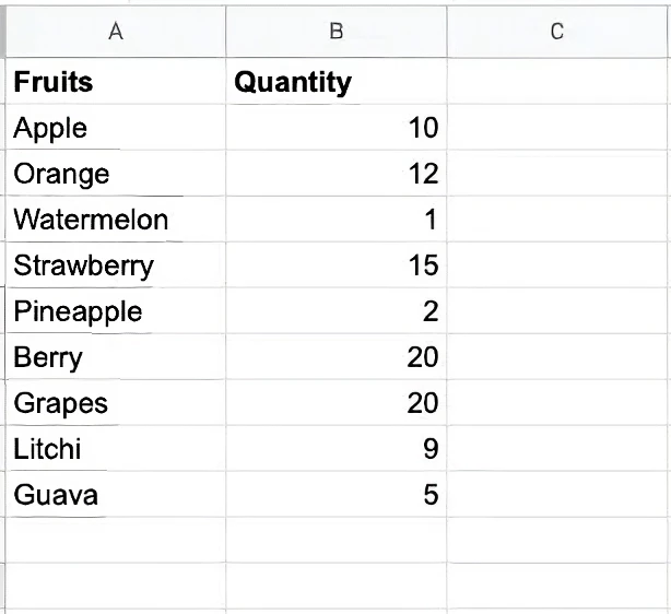
Let’s say you use a lookup function to find the quantity of Mango from your database. Since Mango is not present in your database, you’ll get a #N/A error.
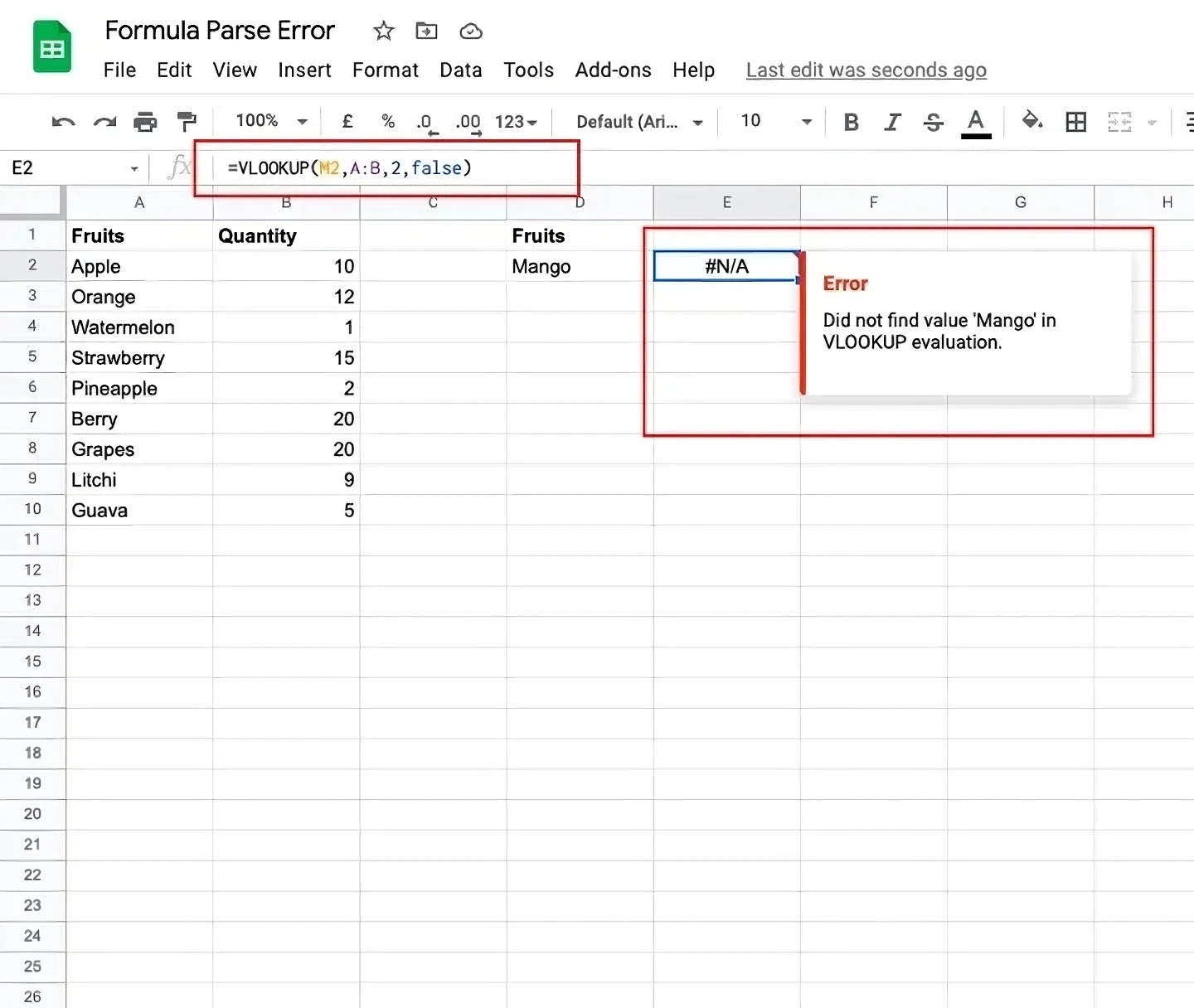
How to fix #N/A
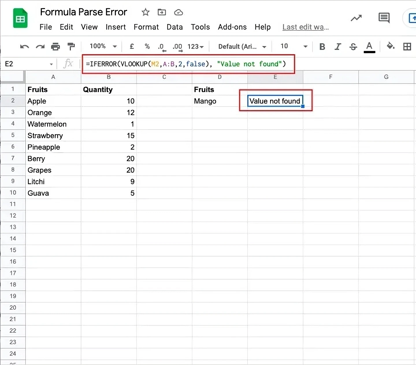
The best way to rectify this error would be to add the missing value to your database or carry a lookup for a different value. However, it would be more helpful if you could display a custom message like “Value not found” instead of showing #N/A. In order to do so, you can use an IFERROR function as mentioned below.
=IFERROR(original formula, value/text to display if there's an error)
For the example above, you can simply replace the existing formula with this:
=IFERROR(VLOOKUP(Search Term,Table,Column Index,FALSE),"Value not found")
#DIV/0!
This error signifies that you’re trying to divide a number by zero in a formula. This can occur when you have a zero or a blank reference in the denominator.
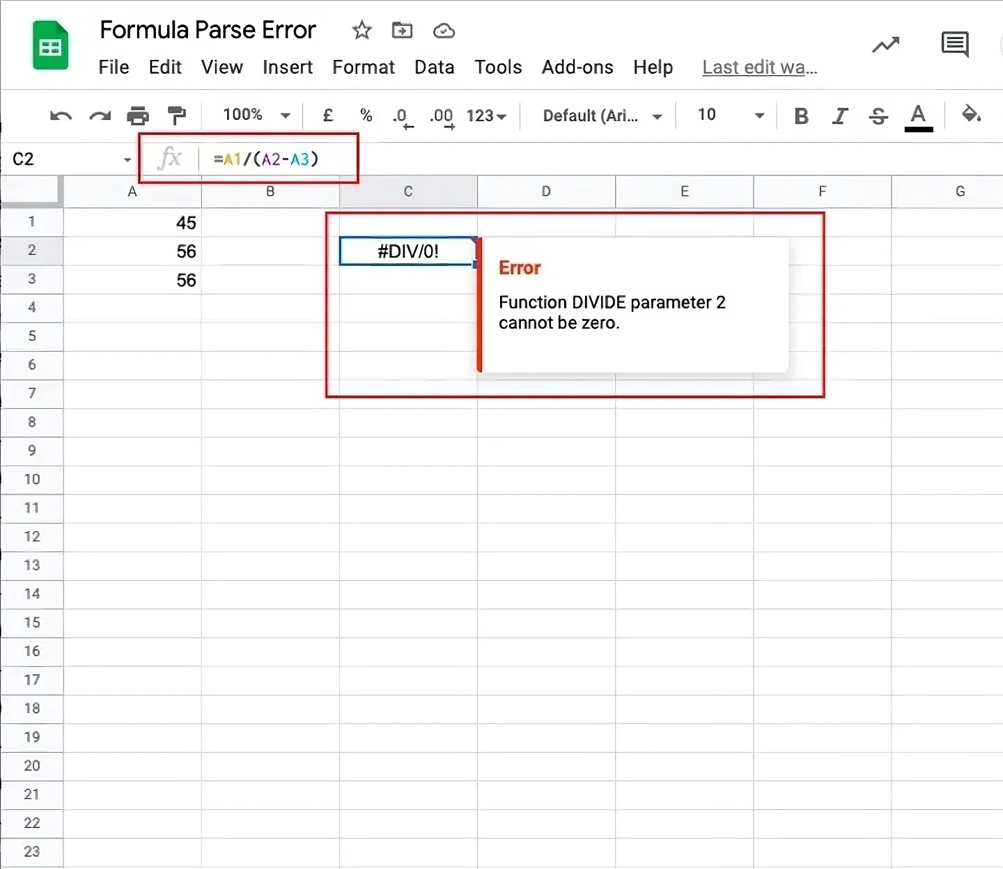
You can also get this error when you try to apply the average function on a range of blank cells.
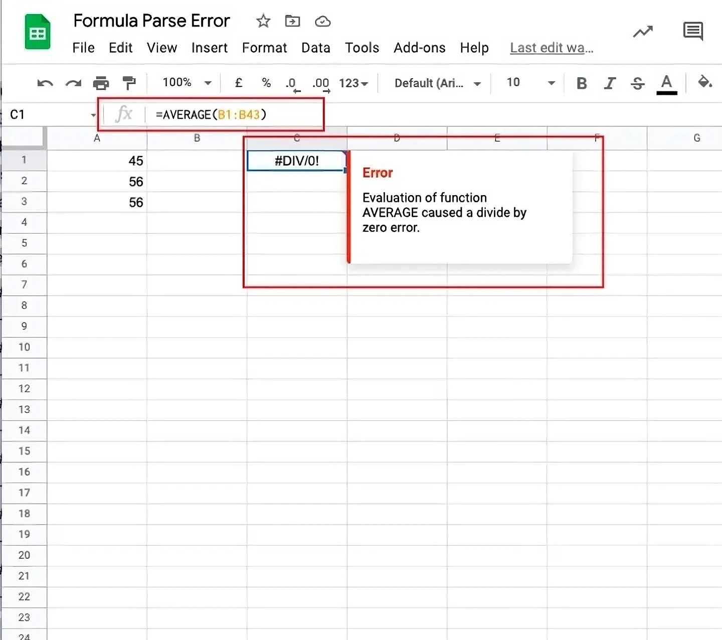
How to fix #DIV/0!
There are a couple of things you could do to fix this error.
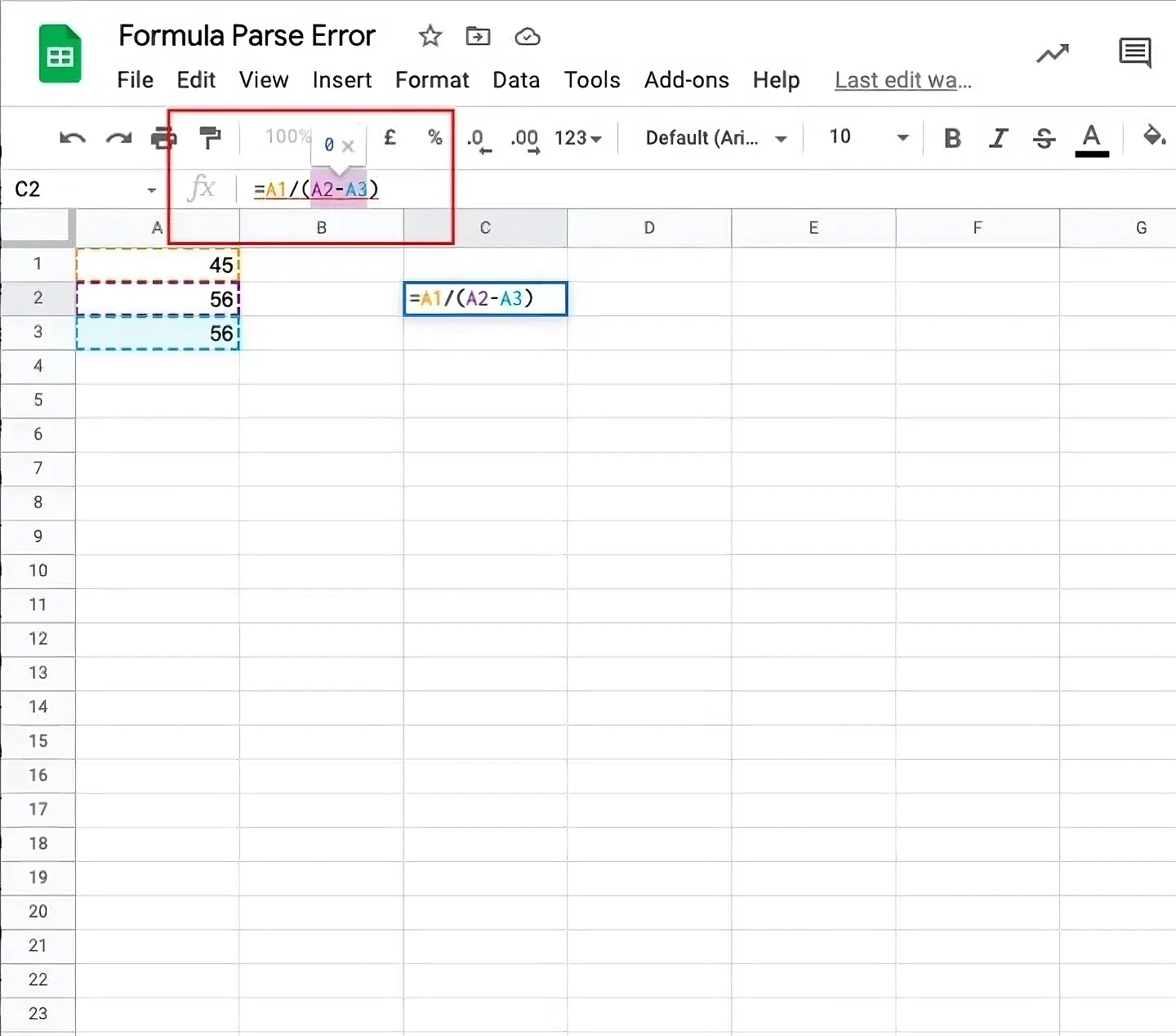
First, you can find out why your denominator in the formula is evaluating to zero. In order to do so, you can select the denominator part in the formula. This will open a little pop-up box containing the result of the calculation right above the formula bar. Once you find the cause, you can make the necessary changes to your formula.
Second, you can check if your denominator in the formula links to a blank range or cell. If true, then you can either fill the blank range or cell with values or select a different range or cell in the formula.
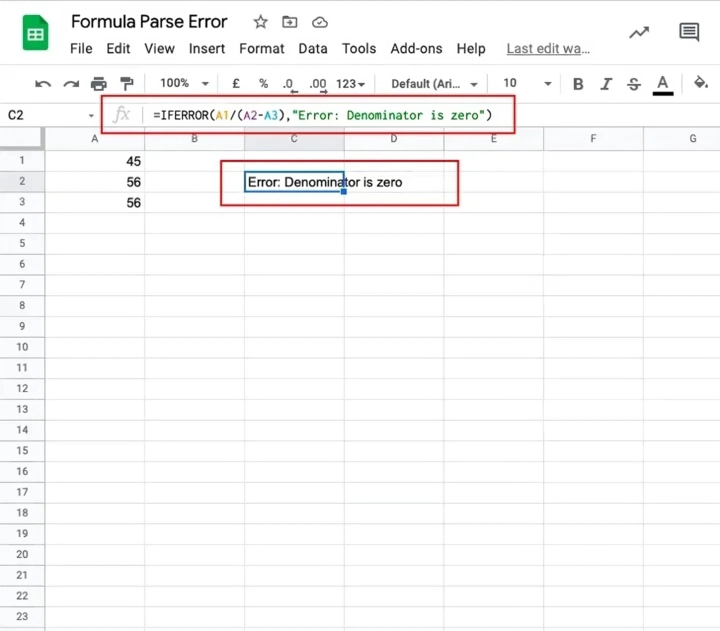
Next, you can also use the IFERROR function as above to display a specific error message when you get a #DIV/0! Error.
#VALUE!
This error occurs when you have a different data type as your input than what is expected in the formula. You’ll get this error if a function accepts numeric data as an argument, but you have a text value in the cell being referenced.
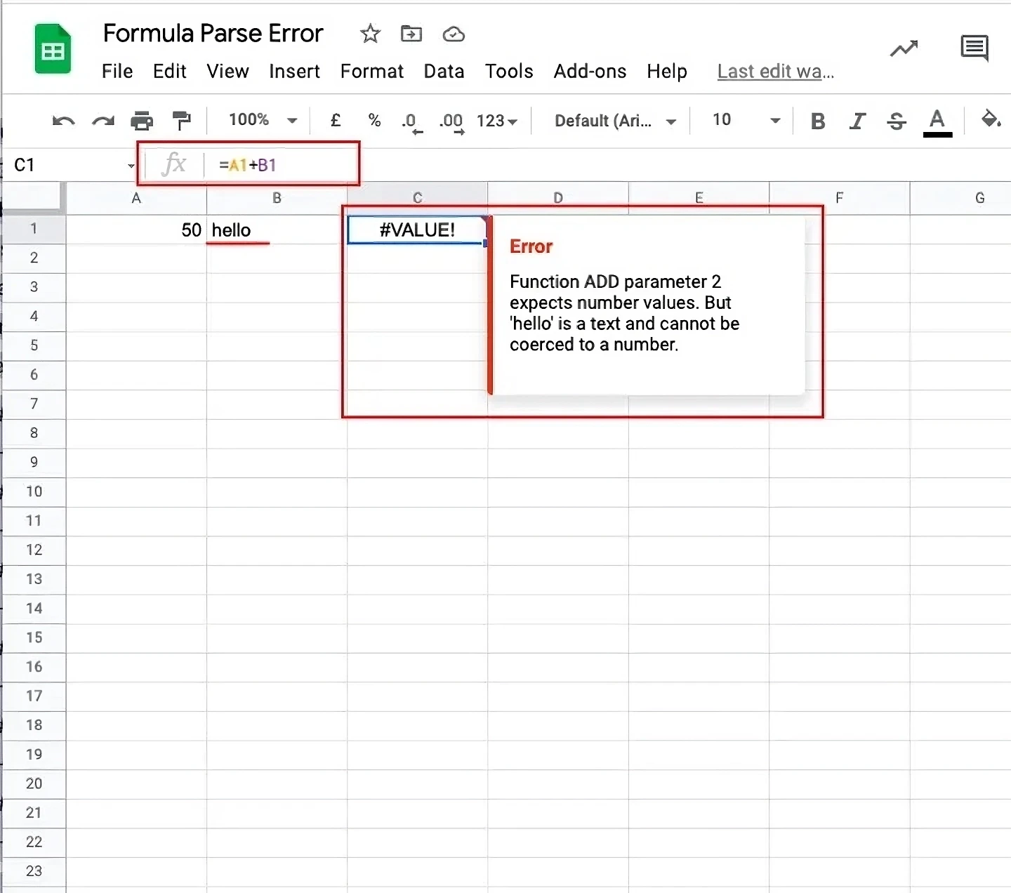
For instance, let’s say you’re trying to add the values contained in cells A1 and A2. However, cell A2 contains a text value instead of a numeric value. Since the parameters of the addition function expect numeric values and we’re trying to add a number to a text, you’ll get a #VALUE! error.
How to fix #VALUE!
If you hover around the cell that displays the #VALUE! error, you can read the error message. This message should give you some idea about the source of the error.
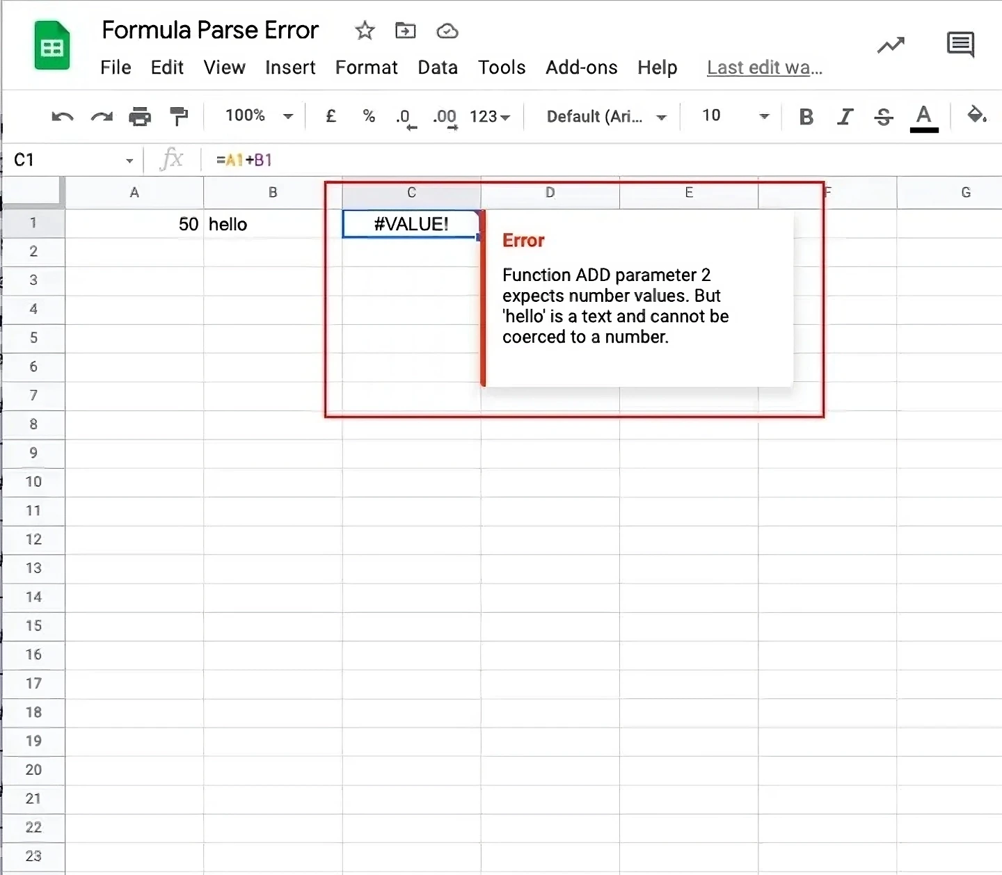
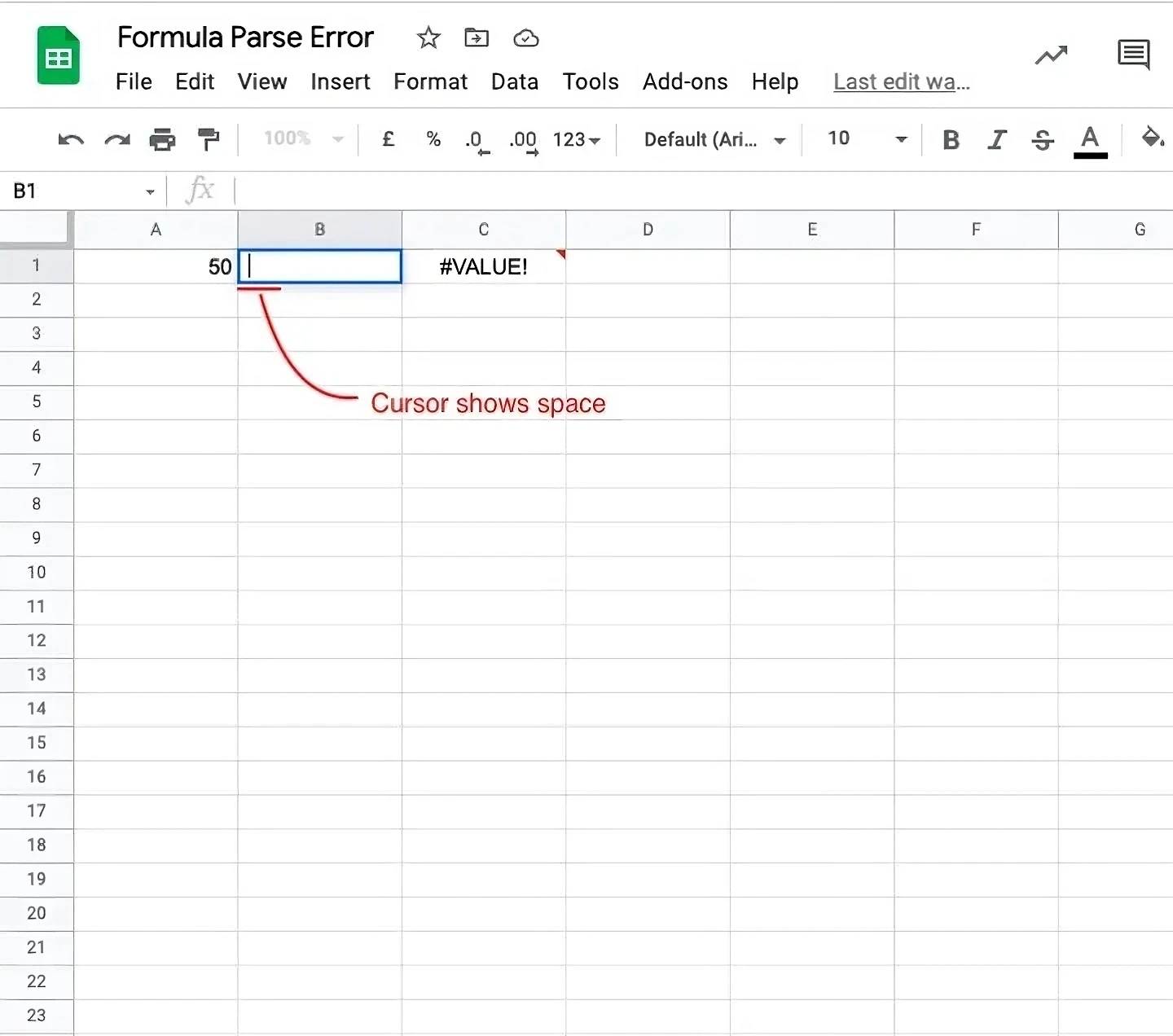
Once you find the source, you can go to the cell or range causing the error and look for errant spaces or any text/number mismatches. It’s easier to get confused between a space in the cell and a blank cell. It is important to note that a blank cell is assumed to have a value ‘0’. However, if the cell has a space in it, then it would be treated as a text. To identify a space, you can click on the cell and see if the flashing cursor has a space between itself and the character next to it.
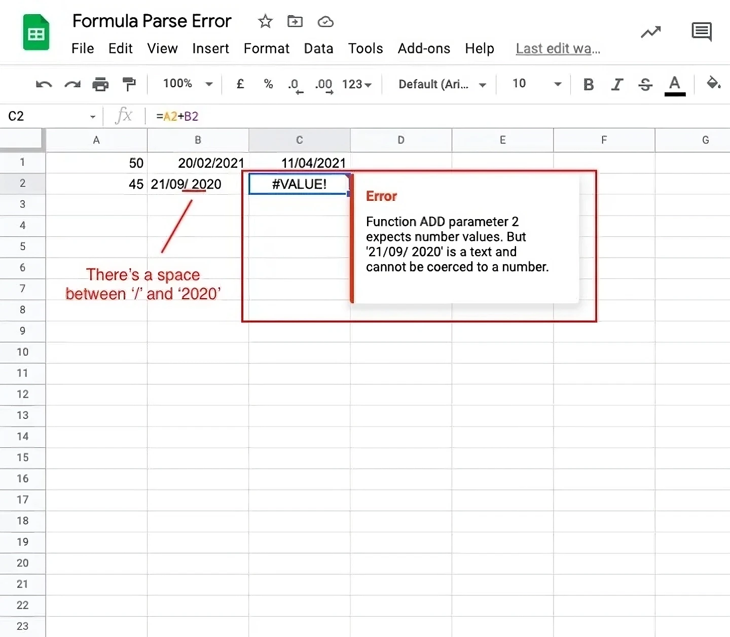
Also, keep in mind that if there are spaces inside a date value or if your date format is not equivalent to the date format DD/MM/YYYY then it would be treated as text. Hence, if you’re using a date in any function and you get a #VALUE! error then chances are that it either contains some spaces or you are using a different date format. So you can check these values and remove any spaces or change the format.
#REF!
This error occurs when you have an invalid reference. There are different types of #REF! errors.
Missing reference: If you reference a missing cell in your formula then you’ll get this error. A cell reference is missing when you delete a row or column in your worksheet. Let’s take an example. Let’s say you want to multiply the values in cell A1 and B1. You use the formula =A1*B1.
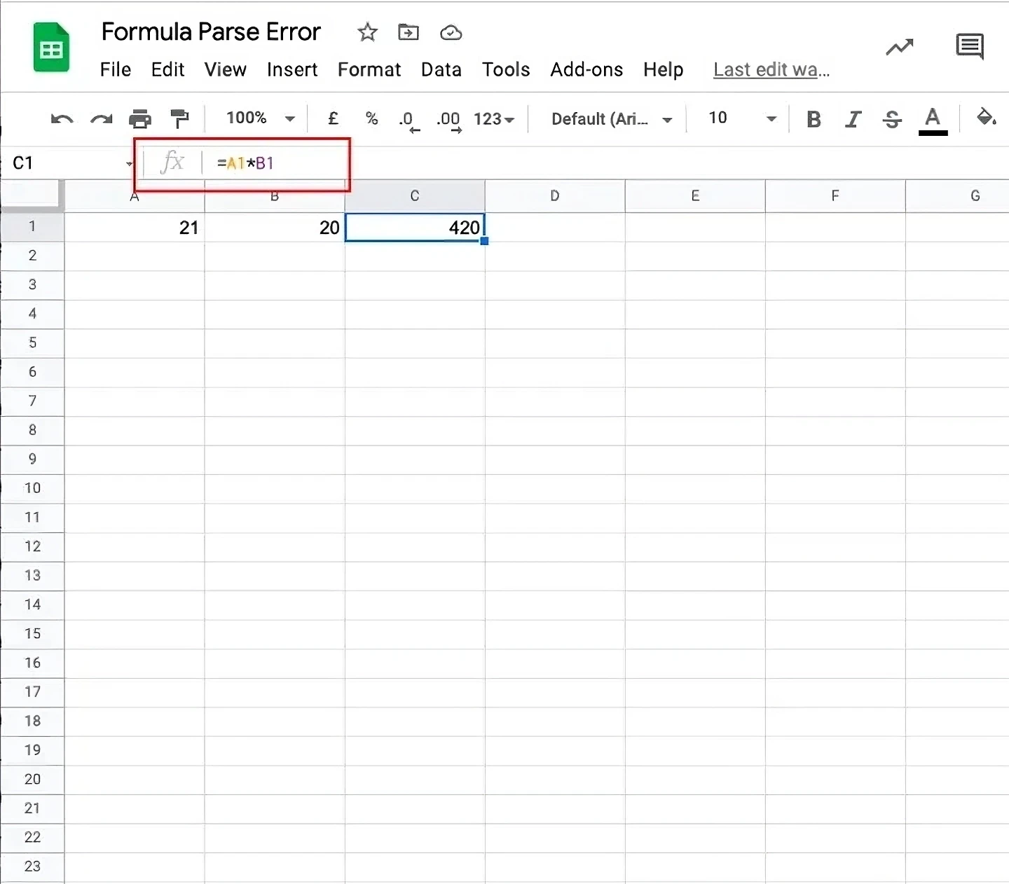
Now, what if you delete the second column of your sheet? Then the value in B1 goes missing. As a result, you’ll end up with a #REF! error.
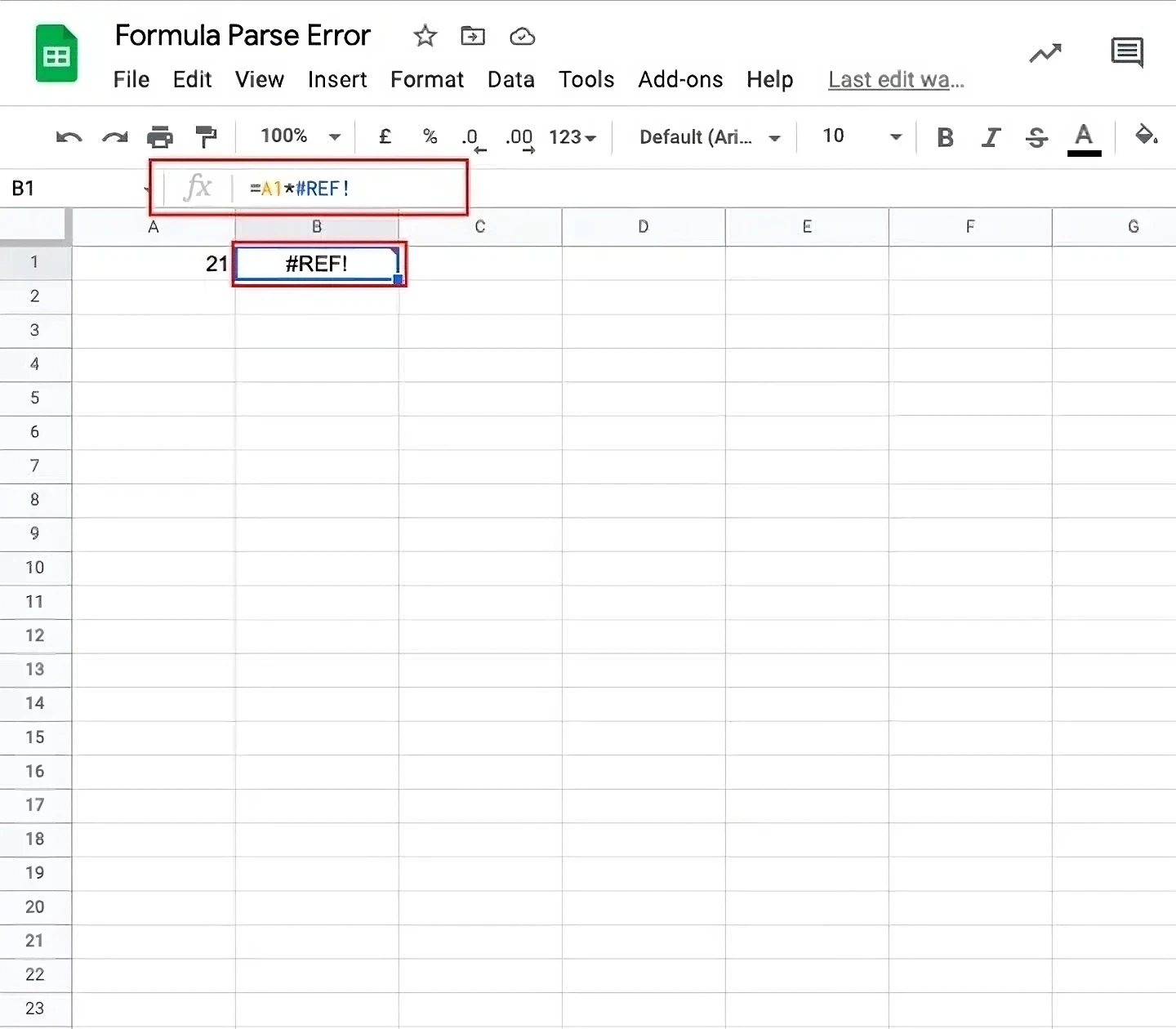
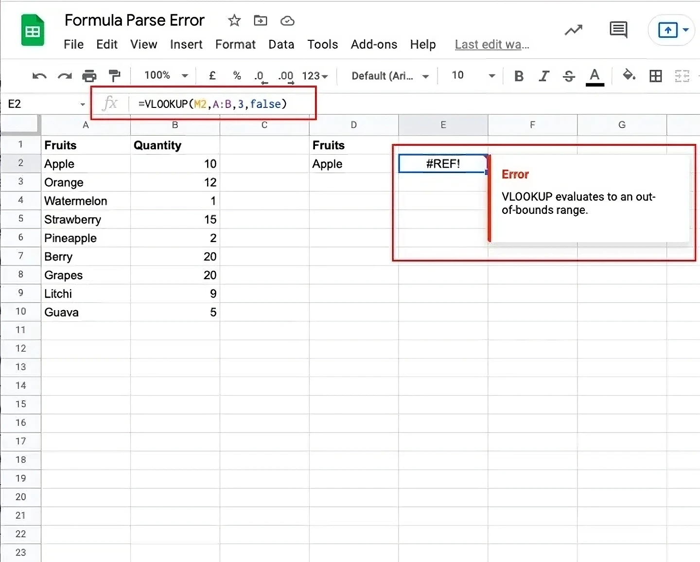
Lookup out of bounds: This error mostly occurs when you’re working with LOOKUP functions. You’ll get this error when you reference a cell that is outside of the range specified in your LOOKUP formulas.
Let’s take the database containing a list of fruits and their quantities as mentioned above. Assume you are trying to use a VLOOKUP function to return a value outside the range specified in the formula. You’ll get a #REF! error.
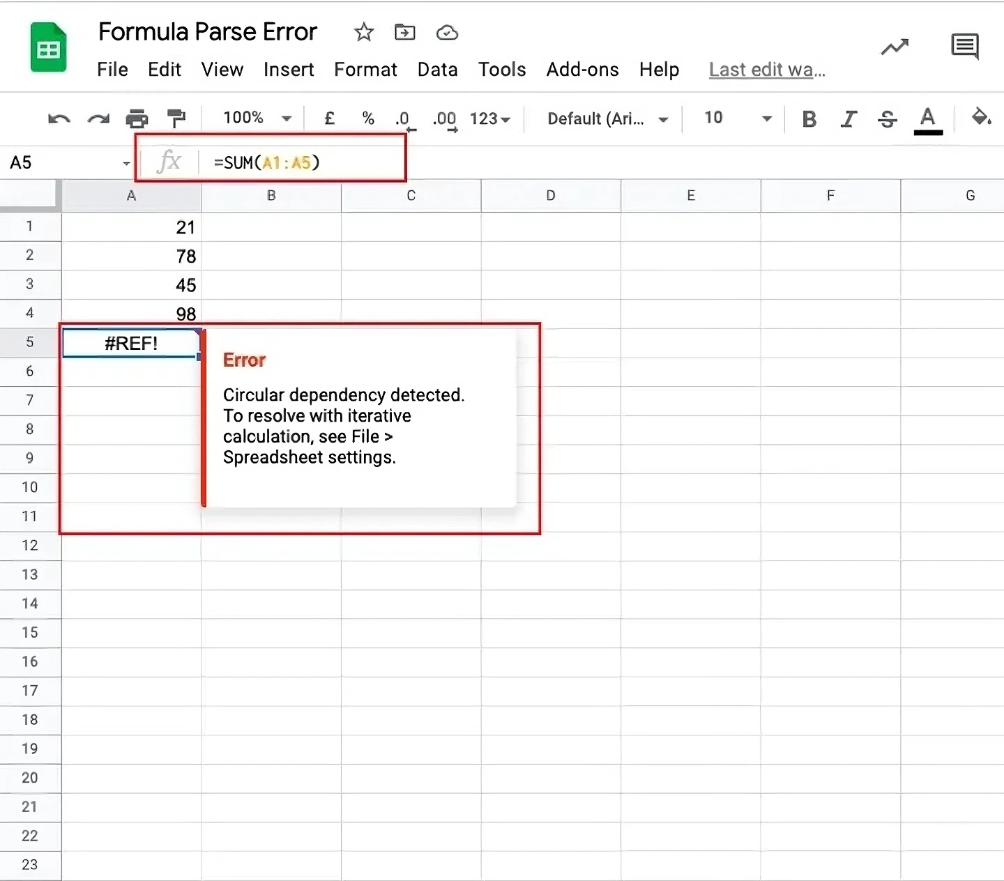
Circular Dependency: This occurs when your formula references itself. Let’s say you’re trying to add the values from cell range A1 to A4 in cell A5. However, instead of using the formula =SUM(A1:A4), you mistakenly use =SUM(A1:A5). Here the cell A5 is trying to be both an output and input. As a result, there is a circular dependency where the value of A5 refers to itself.
How to fix #REF!
The first thing you want to do to resolve this error is read the error message. It gives you an idea of the kind of #REF! error you’re dealing with.
For missing reference, you can search for the #REF! error inside your formula and replace it with the correct cell reference.
For lookup out of bounds, you can either change the range or the search term itself in the formula. You’d have to make sure that the search term exists in the specified range.
For circular dependency, identify the cell that’s causing the problem from the range of cells in the existing formula. Then modify it such that the range doesn’t include the current cell in it.
Improve your DTC game. Sign up for weekly tips.
#NAME?
This error occurs when the syntax of your formula is incorrect. Below are the images of some of the common mistakes people make that generate this error.
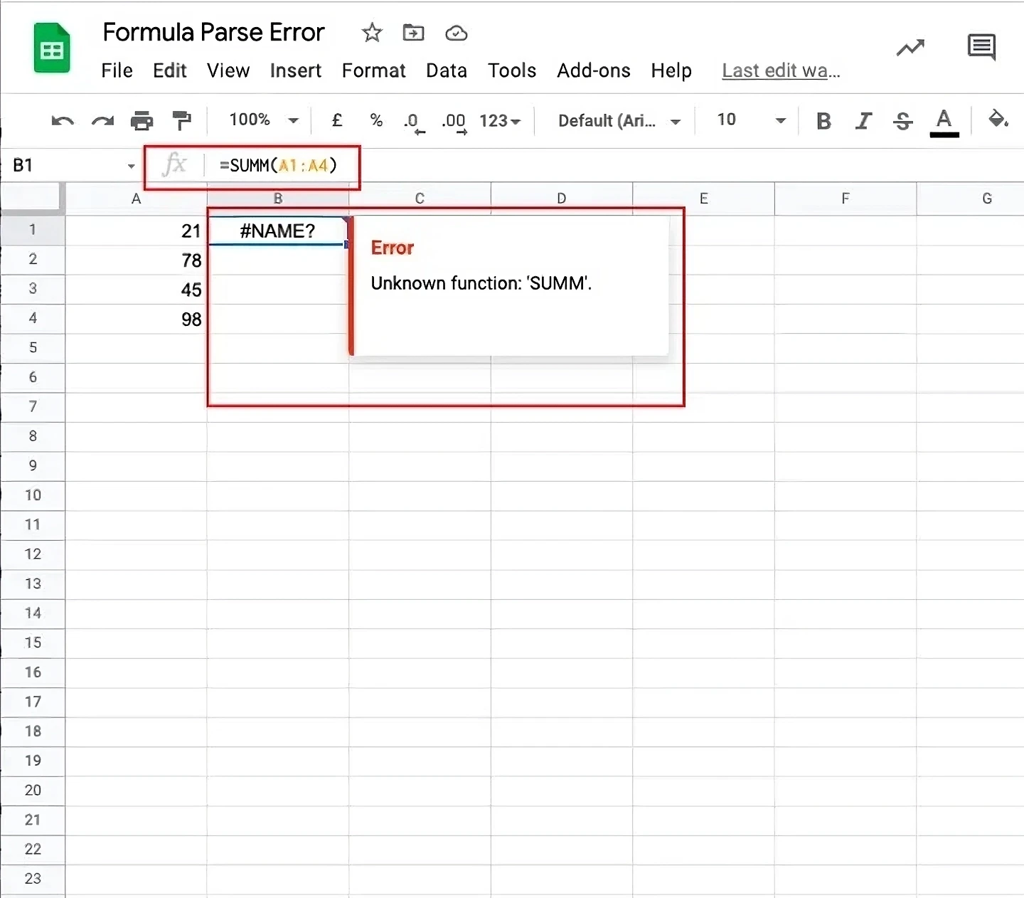
The first is a spelling mistake. If you mistakenly misspell the name of the functions or the range then you’d get this error. In the image below, you can see a #NAME? error after misspelling the function SUM.
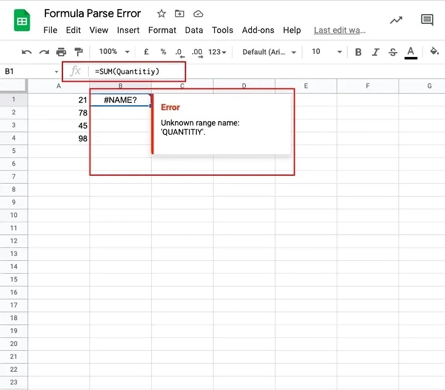
The second is an incorrectly named range. If you try to refer to a range that does not exist then you’ll get this error. In the image below, we’re trying to use the SUM function in a range of cells named Quantity that doesn’t exist.
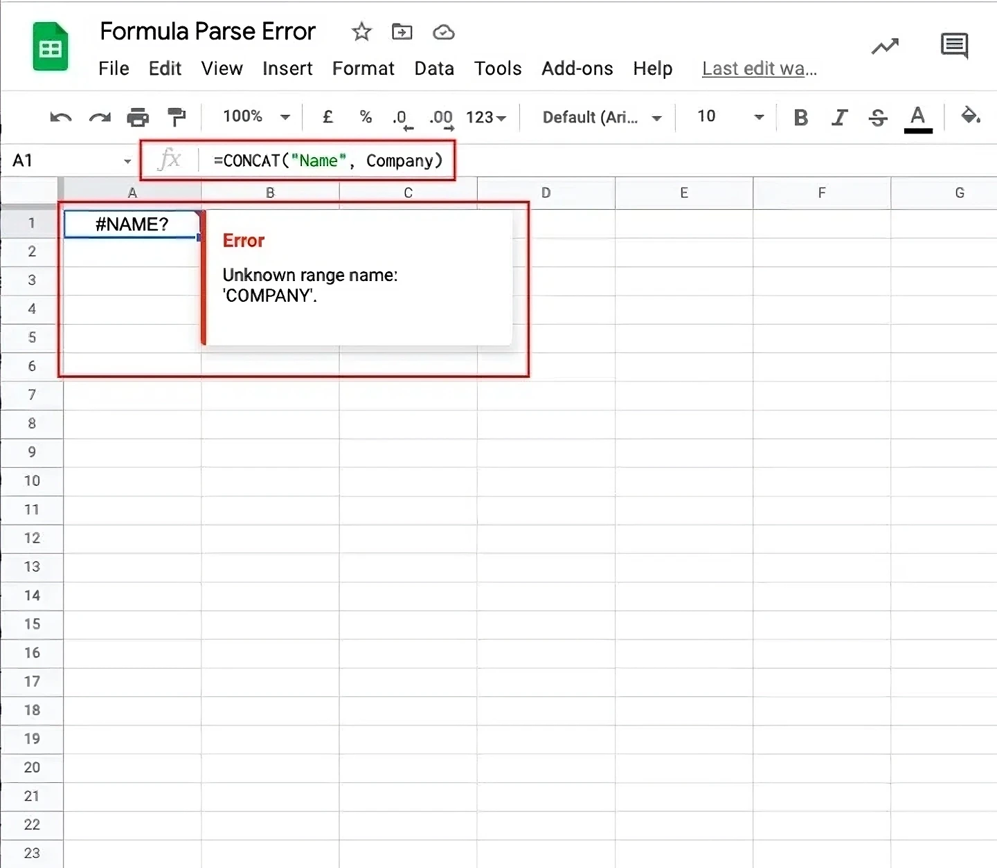
The third is the presence or the absence of quotation marks in the formula. If you forget to add quotation marks where required then you’ll end up with a #NAME? error as shown below. In the image below, there are no quotation marks for the word “Company” inside the CONCAT function. As a result, we got a #NAME? error.
How to fix #NAME?
The best way to resolve this error is by checking if there are any spelling mistakes in the function names or range names. You can also check if the string values are enclosed with quotation marks in your formula.
#ERROR!
This is a unique type of error that occurs when Google Sheets cannot understand your formula. There are many reasons why you may get this error.
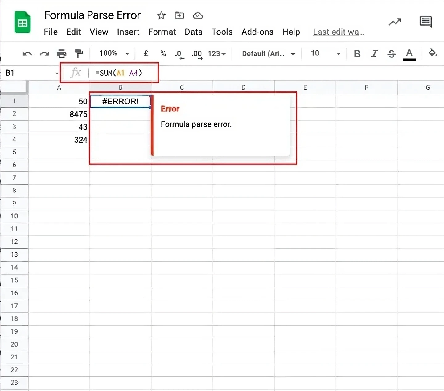
One of the reasons you could get this error is when you forget an important operator in your formula. For eg, forgetting to add a colon while denoting the range or a comma between cell references could yield this error.
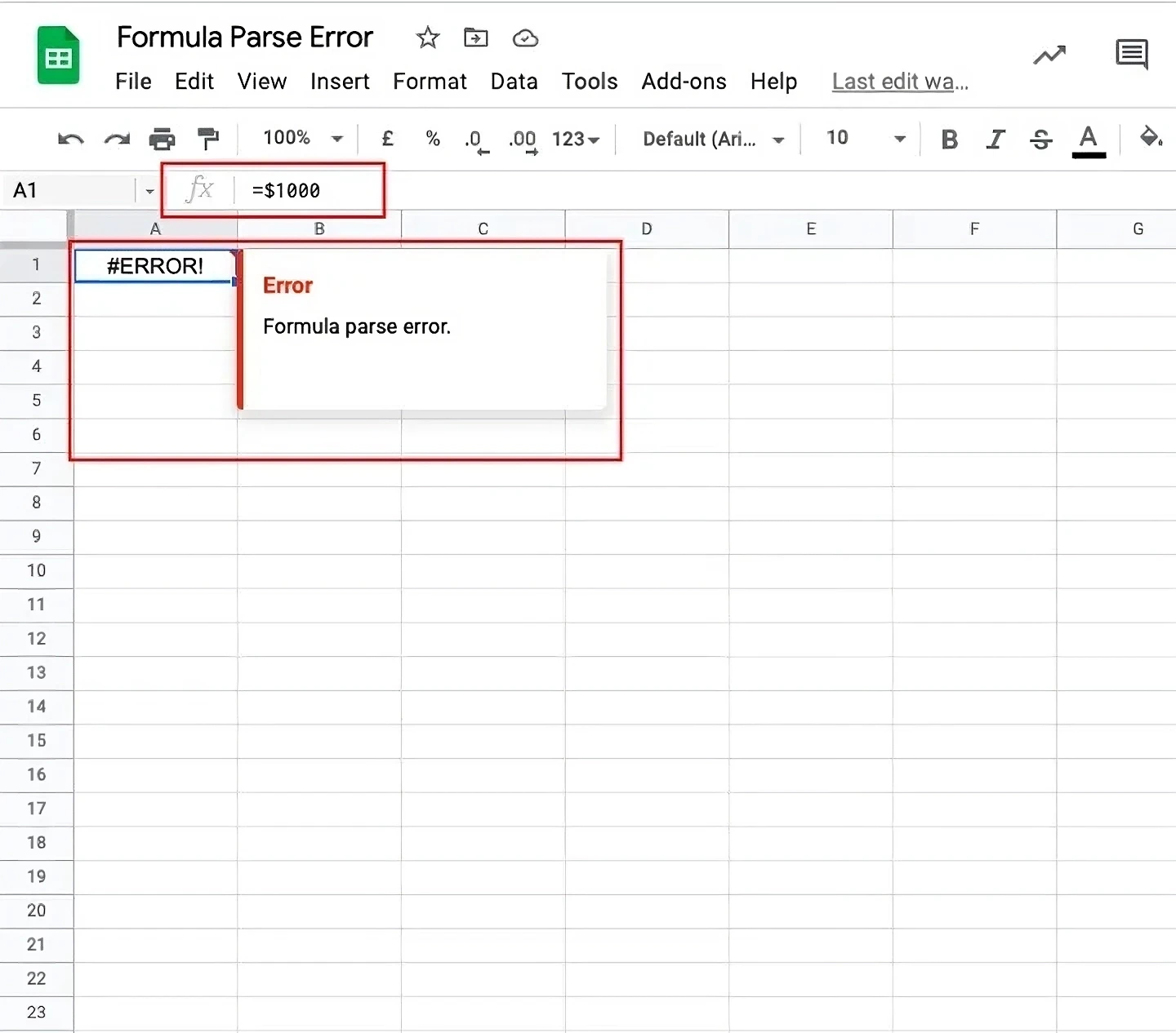
Another reason could be that the opening brackets do not match with the closing brackets in your formula or that you've manually typed $ in your formula to indicate an amount. Adding a $ sign would mean that you’re indicating a cell reference, hence, you'll get an error.
How to fix #ERROR!
It might be quite tedious to resolve this error especially if you’re working with long and complex formulas. Having said that, you can lookout for a few things in your formula when you get this error.
You can check if you’re missing out on any operators in your formula.
You can check if the number of opening brackets matches the number of closing brackets.
You can check if you’re using any currency like $ to denote the amount in your formula. If true, then the currency needs to be removed.
These are some of the most common formula parse errors in Google Sheets. Having said that, this is not an exhaustive list. There are many other kinds of formula parse errors that we have not covered in this blog. But for almost all the formula parse errors, it is important to note that they can be resolved no matter how frustrating it might be to deal with them. You’d first have to figure out what the error is trying to signify. Once you find the source and cause of the error, you can easily fix it by making necessary changes.


