Reporting & Analysis
25.11.2021
TLDR
Google Sheets' conditional formatting can help improve data readability. You can highlight specific values in a column, find and highlight duplicates, highlight blank cells, locate cells with errors, and dynamically highlight cells containing a search string.
There's a lot of fun stuff you can do to make your GSheet tables look better.
Last week, my colleague Sona Maharjan talked about how to merge cells and data to make your tables look cool. Conditional formatting is another easy way to format your data for easy reading. In this guide, we will go through the most common uses of this feature.
Remember to bookmark this guide to grab the custom formulas when you need it next.
These are the scenarios we will go through:
How to highlight cells with specific values, using conditional formatting.
How to highlight duplicate values with conditional formatting.
How to highlight cells with errors using conditional formatting.
How to dynamically highlight cells that contain a search string.
How to highlight cells with specific values.
Let's get started. Here we have a a table with two columns—one containing random numbers and another containing names. We will try to highlight the cells in the names column that contain certain names.
First, highlight the column where you wish to apply the conditional formatting, then go to Format → Conditional Formatting.
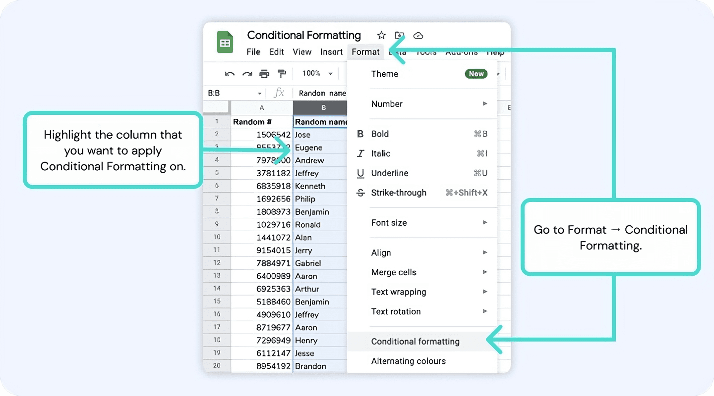
This will open up a sidebar showing you the conditional format rules. Let's say we want to highlight all the cells on the second column that contains the name "Benjamin". Under the Format rules section, let's use the dropdown to select Text Contains and type in Benjamin in the space provided.
You can also select the color you want to use to highlight the cells. Here's what the output looks like.

How to highlight duplicate values using conditional formatting.
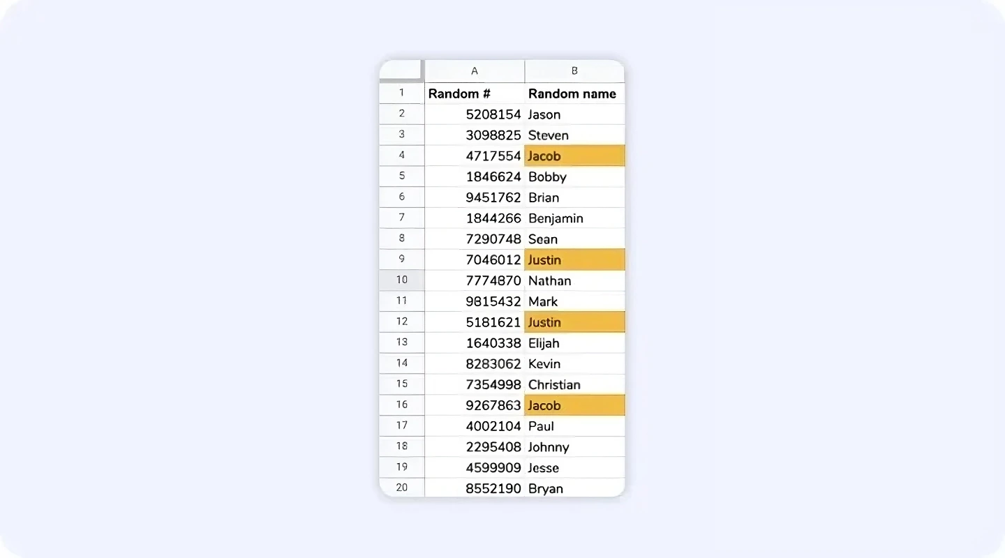
This time, let's say we want to highlight cells that have the same value repeated two or more times. Unlike MS Excel, highlighting duplicates is not a default option in Google Sheets. So, we are going to use the Custom Formula option to highlight those cells instead.
Choose the right column and go to Conditional Formatting again. This time, click on the dropdown under Format Rules and select Custom Formula Is. Then type in the following:
=COUNTIF($B$2:$B,B1)>1
That's it! Select the color you wish to use to highlight the duplicate values and you're done!
Here's the final output.
How to highlight blank cells using conditional formatting.
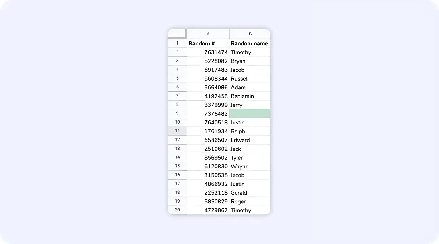
There are a couple of ways to do this, but the easiest way is to simply select the 'Is Empty' option from under Format Rules.

You can also use the Custom Formula option to highlight blank cells as well. Again, highlight the column you wish to apply the conditional formatting to, go to Format → Conditional Formatting and select custom formula from the Format Rules dropdown. Then type in the following:
=ISBLANK(B2)
This will highlight all the cells in the column B that are empty. Here is the output you will get.
Improve your DTC game. Sign up for weekly tips.
How to highlight cells with errors using conditional formatting.
Sometimes when you have a long list of entries, it's best practice to first find any errors that may have been generated by formulas. If you have thousands of rows, you can't simply glance through to find errors.
To find cells with errors, first go to Format → Conditional Formatting and select custom formula from the Format Rules dropdown. Then type in the following:
=ISERROR(B2)
That's it! This will highlight all your cells with errors in red, making them easier to find and fix. This is the final output you can expect.
How to dynamically highlight cells that contain a search string.
Sometimes you want to find a specific cell that contains a search string you enter elsewhere. You can create filters to search for that search string, or go the Control + F route, but it is a better user experience to do this with conditional formatting.
We will create a reference cell where you can type in the search string (say, the names on Column B in the example above). This is the outcome we're shooting for.
It's simpler than it looks: I promise (well, sort of). Same as before, highlight the column you want to format, then go to Format → Conditional Formatting and select custom formula from the Format Rules dropdown. Type in the following:
=AND(NOT(ISBLANK($B$2)),ISNUMBER(SEARCH($B$2,B3)))
That's it! Choose the right color for yourself and you get your search working just like the video above. 🎉
Are there other scenarios you would like to use Conditional Formatting on? Let us know on hey@airboxr.com and we will add to this definitive guide! 🎉


