Reporting & Analysis
Feb 9, 2022
TLDR
XLOOKUP is a powerful function in Microsoft Excel, available to Microsoft 365 users, that allows you to search and retrieve data both vertically and horizontally. It's a replacement for functions like VLOOKUP and HLOOKUP. You can use it to find values based on lookup criteria and handle unmatched values as needed. While XLOOKUP isn't available in Google Sheets.
An advanced LOOKUP function. Plus an alternative for Google Sheets.
Excel released a powerful LOOKUP function called XLOOKUP in 2019. It can perform a lookup both vertically and horizontally, hence, is meant as a replacement for Excel’s existing LOOKUP functions: VLOOKUP, HLOOKUP, INDEX/MATCH.
In this article, we will go over everything you need to know about the XLOOKUP function, along with some examples.
What is XLOOKUP function?
XLOOKUP function in Microsoft Excel allows you to search for an item in a vertical or horizontal range and return its corresponding value. Unlike VLOOKUP/HLOOKUP, XLOOKUP can lookup data in any direction of lookup values.
XLOOKUP can lookup data in any direction of lookup values.
How to get access to XLOOKUP?
XLOOKUP is only available for the users of Microsoft 365. If you are using Microsoft 365 suite on your computer, then this function will be automatically enabled on your Excel.
If you’re on older Microsoft 365 edition, such as home, personal or university and can’t access XLOOKUP function, then you can follow these steps:
Go to File → Account
Join the Officer Inside Program
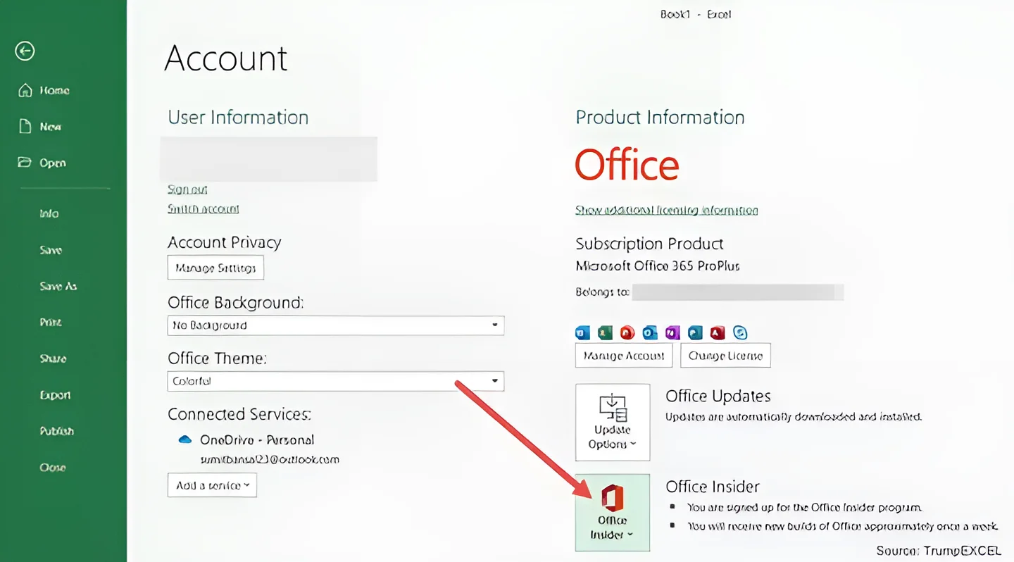
If you’re not on Microsoft 365, then you might need to upgrade your version to access XLOOKUP.
Click here to upgrade to Microsoft 365
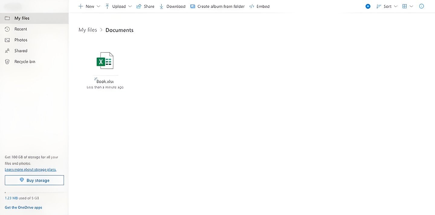
You can also access XLOOKUP from online Excel. To do so, you would first have to sign into OneDrive on the web. Then either create a new excel sheet or upload your existing excel file in your OneDrive folder.
Syntax for XLOOKUP function
=XLOOKUP(lookup_value, lookup_array, return_array, [if_not_found], [match_mode], [search_mode])
XLOOKUP function takes up to six arguments.
lookup_value (required): the value to search for
lookup_array (required): the array or range to search for the lookup value.
return_array (required): the array or range to return your matching value from
[if_not_found] (optional): return this value when the match isn’t found
[match_mode] (optional): specify your match type
[search_mode] (optional): specify the search mode
Values you can use for [match_mode]:
0 (default): Exact match. If not found, return #NA.
1: Exact match. If not found, return the next larger value.
2: A wildcard match where *, ?, and ~ have special meaning.
Values you can use for [search_mode]:
1 (default): Perform a search starting at the first item.
-1: Perform a reverse search starting at the last item.
2: Perform a binary search where the data needs to be sorted in ascending order. If not sorted, return invalid.
-2: Perform a binary search where the data needs to be sorted in descending order. If not sorted, return invalid.
How to use the XLOOKUP function
Let’s take a look at a few examples to get a better understanding of how to use XLOOKUP.
Example 1: XLOOKUP to fetch a lookup value vertically
For the purpose of this blog, we’ve created a table containing customer data of a store as shown below. Let’s assume we want to find the total amount spent by the customer Christian.
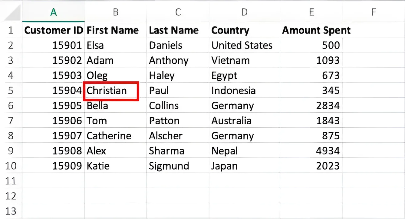
Let's look at the format we want the output to be in. We have the customer’s name with the amount spent in a new table shown below:
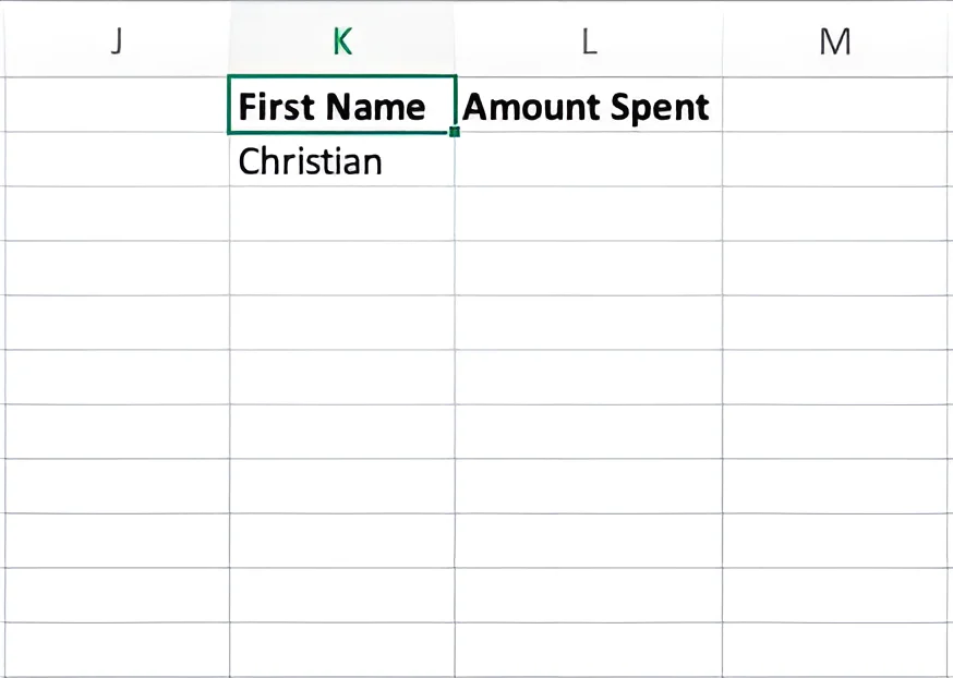
We want to display the amount spent by Christian in cell L2. Now let’s go to L2 and type in the following formula.
=XLOOKUP(K2, B1:B10, E1:E10)
OR,
=XLOOKUP("Christian", B1:B10, E1:E10)
Here, K2 or "Christian" is the lookup_value, B1:B10 is the lookup_array and E1:E10 is the return_array. You can use either a cell reference or a string as a lookup value. If you’re using a string, it should be enclosed in quotes.
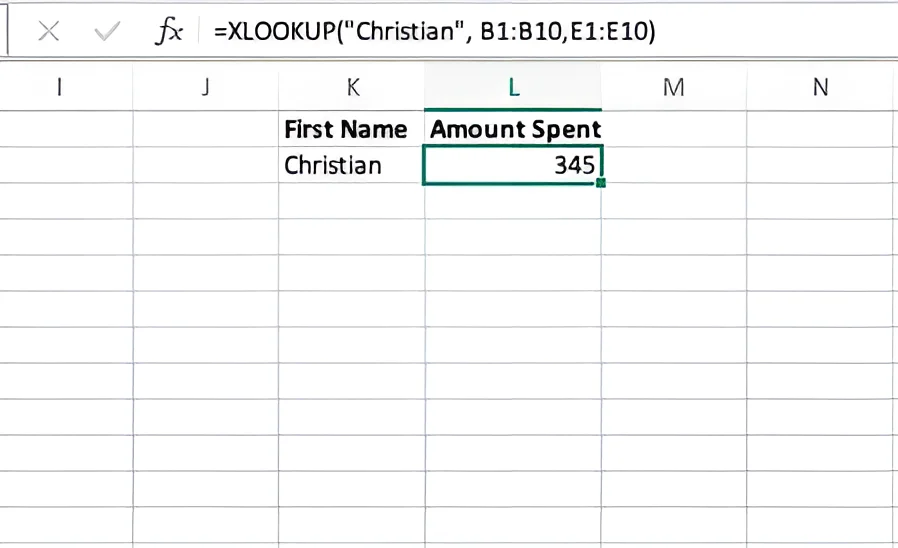
Now, let’s see what happens when return_array is on the left of lookup_array.
Let’s take the same dataset but with the first name column on the right.
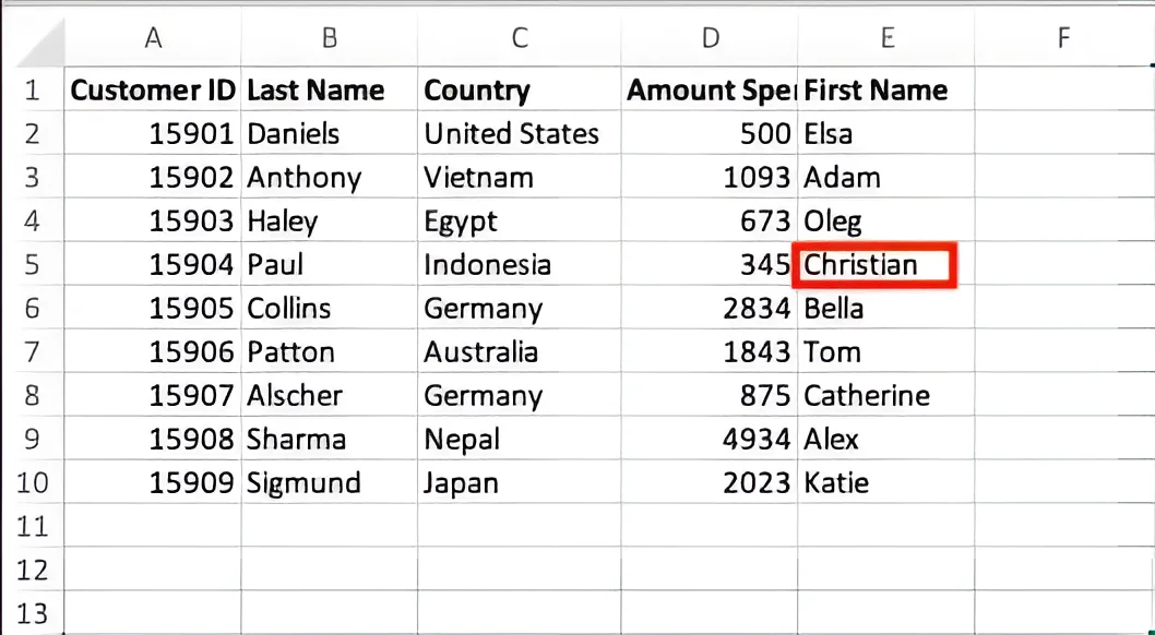
Here we're trying to perform a lookup to the left of the lookup value. Let’s use the following formula.
=XLOOKUP("Christian", E1:E10, D1:D10)
We will still get the same result.
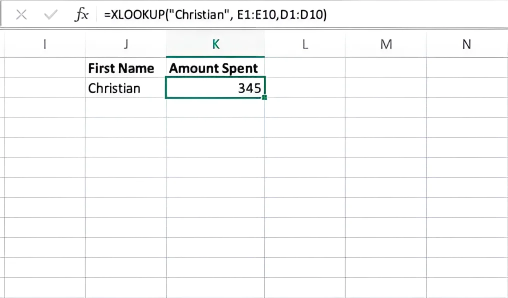
XLOOKUP addresses one of the major issues with the VLOOKUP function. You can move the rows and columns around, and XLOOKUP would still work. VLOOKUP would have thrown an error.
Example 2: XLOOKUP to fetch multiple values
With XLOOKUP, we can also fetch multiple values. Suppose we want to get the values of Christian’s country name and the amount spent. We can use the following formula.
=XLOOKUP("Christian", B1:B10, D1:E10)
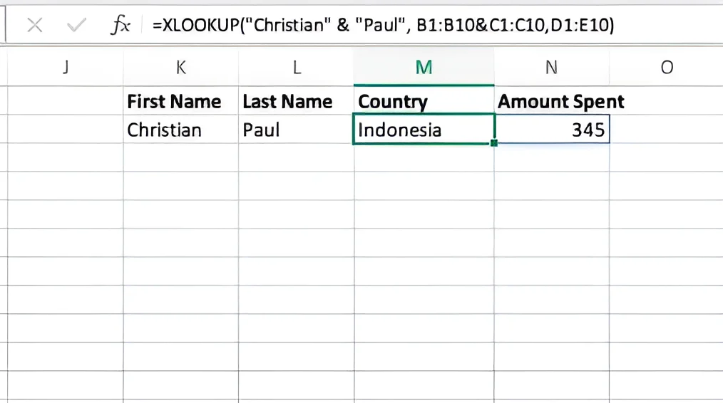
Here, the formula uses a return_array that contains a range of two columns (D1:E10). Therefore, when the lookup value is found in the lookup_array (B1:B10), the formula returns the values of the entire row from the return_array.
Improve your DTC game. Sign up for weekly tips.
Example 3: XLOOKUP with multiple criteria
XLOOKUP also allows you to perform lookups when you have more than 1 criterion. Let’s take the same dataset as above. Now assume you want to find out the amount spent by Christian Paul. Our dataset has separate columns for first and last names. So to perform this query, you would have to look up both the values Christian and Paul in the dataset. With XLOOKUP, this can be done easily.
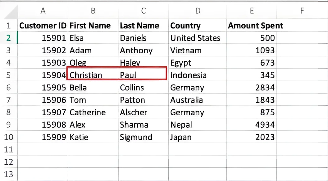
We can simply type the following formula in the required cell.
=XLOOKUP("Christian" & "Paul", B1:B10 & C1:C10, D1:E10)

Here, the formula uses two lookup values ("Christian" and "Paul") and two lookup arrays ( B1:B10 & C1:C10). It is important to note that when using multiple criteria, you need to add the required lookup values and lookup arrays using an ampersand (&).
Example 4: XLOOKUP to fetch a lookup value horizontally
Now let’s take a look at how XLOOKUP can be used to look up horizontally. For this example, we have transposed the above dataset. So the new dataset looks like this.

Let’s take the same case as shown in Example 1. We want to find the total amount spent by the customer Christian. We can use this formula.
=XLOOKUP("Christian", A2:J2, A5:J5)
Here, instead of a vertical range, we have a horizontal range for both lookup_array and return_array.
XLOOKUP is a powerful LOOKUP function that can help you search through your Excel spreadsheets in an instant. It does not exist in Google Sheets yet. So if you’re someone who prefers working with Google Sheets over Excel, you’d still have to work with older LOOKUP functions.


