Reporting & Analysis
Feb 2, 2021
TLDR
To create a pivot table without column or row names, follow these quick steps: First, go to Data → Pivot Table and select a new sheet. Then, add the relevant data to Rows and Values in the Pivot Table Editor. You can change the summarization method if needed. Finally, you can filter data to exclude specific rows.
And how to interpret data the correct way.
Using pivot tables is a quick way to get your data organized for analysis. Here are some quick instructions on putting together a pivot table that helps arrange your data properly.
Let's start with this dummy data of items ordered on a Shopify store. Using the raw data on the left, we will build the pivot table on the right.
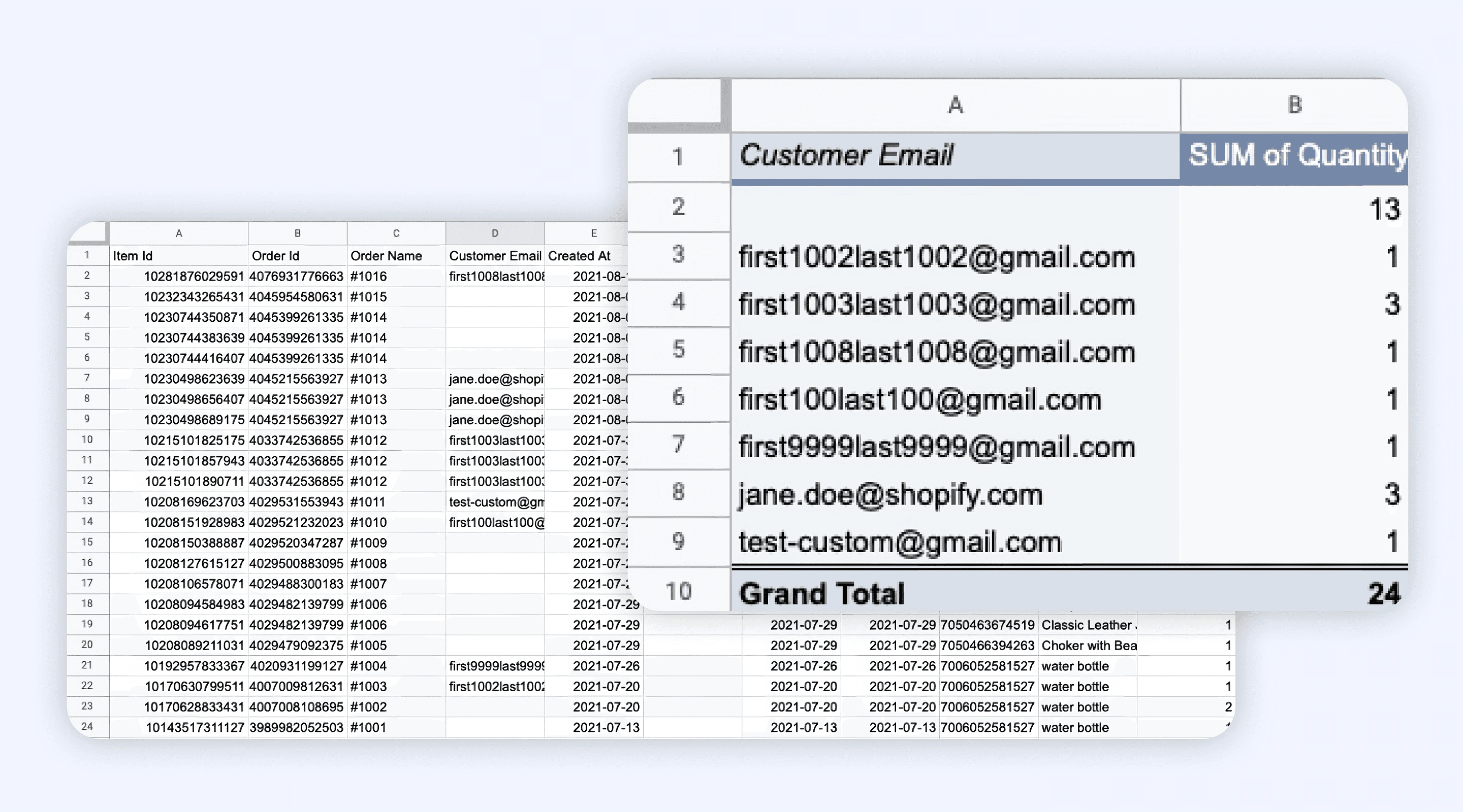
You can see here that some of the cells in the raw data sheet are blank. They're supposed to have the customer's e-mails but they don't—maybe the customer didn't enter an e-mail to make her purchase. This will become important later; for now, file this away.
Launch the Pivot Table Editor
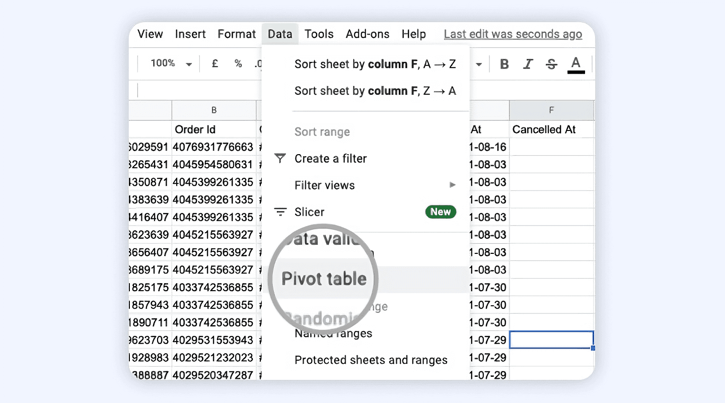
Go to Data → Pivot Table from the top menu and launch the pivot table builder. When you launch the pivot table editor, you will be asked if you wish to create your pivot table in a new sheet or an existing sheet. For convenience, we will select a new sheet.
Set up your Pivot Table
This will create a new sheet for you with a blank pivot table and launch your pivot table editor.
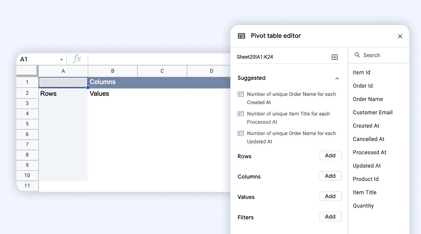
Click the Add button next to Rows and select Customer Email
Click the Add button next to Values and select Quantity
Your Pivot Table Editor should look something like this. Note how the values are being summarized as Sum. You can change it to another summarization (e.g., average etc.)—but sum makes sense in our context here since we want the total quantity of products purchased by each user.
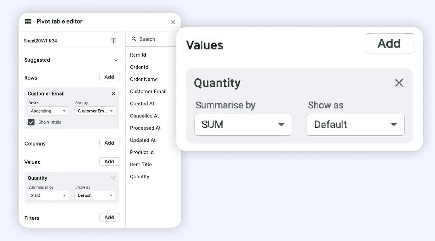
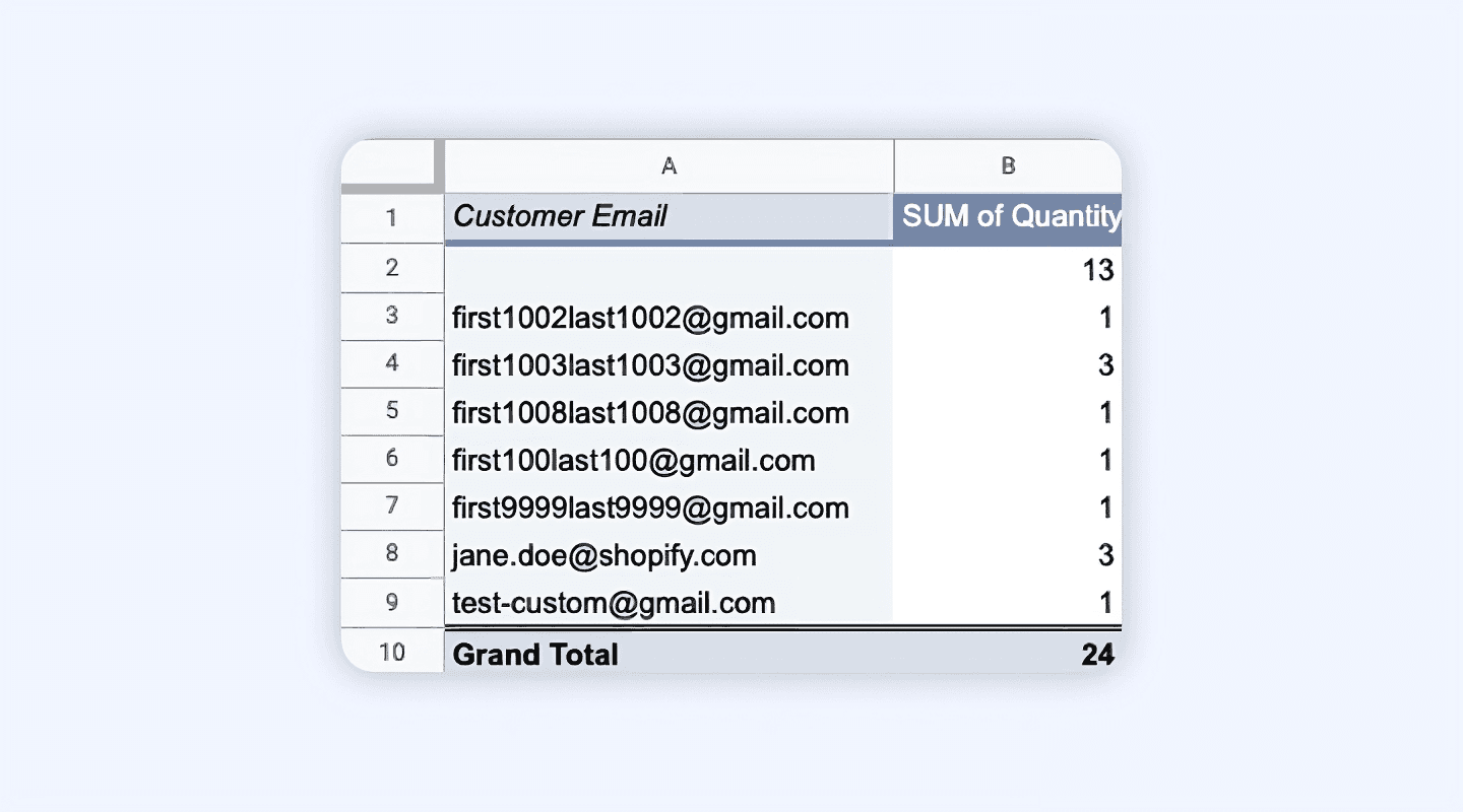
That's it, as you go through the steps, you will see your pivot table populate with the numbers. The final output should look something like this.
Improve your DTC game. Sign up for weekly tips.
One quick note.
You may notice here that the 13 items were ordered by customers with no email. This could mean a lot of things—there might be one customer (without an email) who ordered 13 items or 13 customers who ordered one item each. Make sure to take that into account when interpreting data on your pivot table.
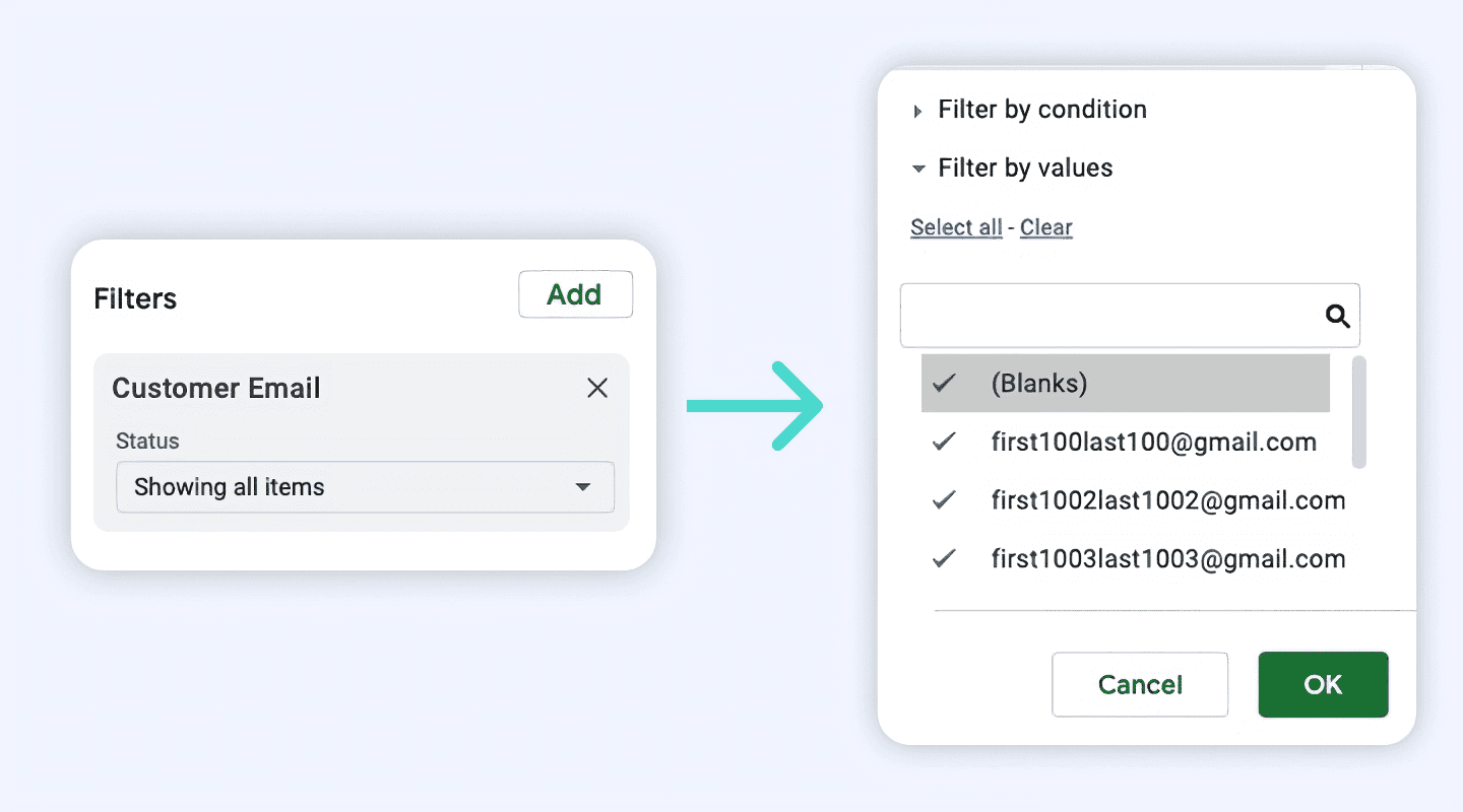
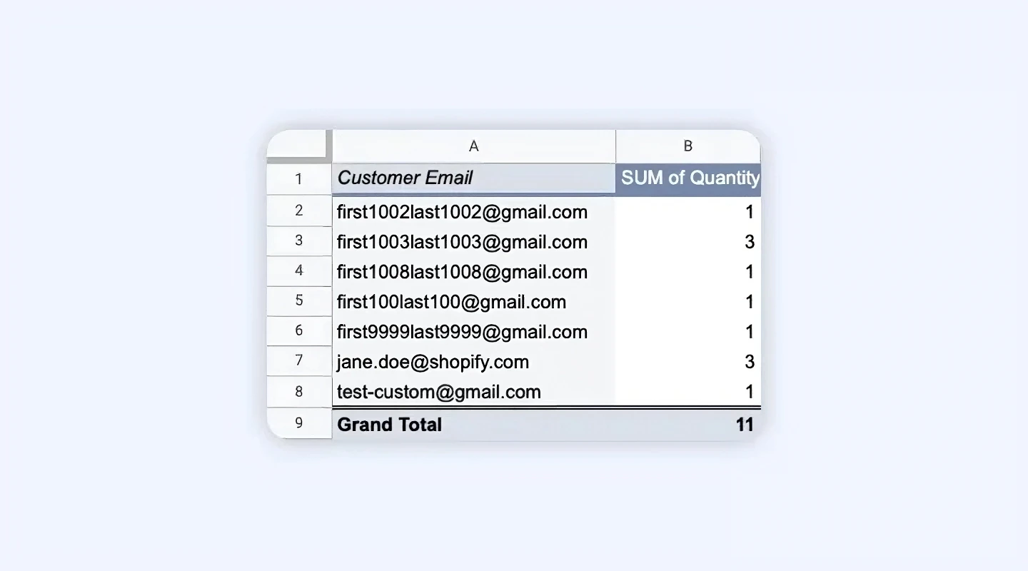
If you want to look at customers who have email addresses and ignore the rest, you can use the Filter option on the Pivot Table Editor to remove customers without emails. Simply click Add next to Filters, then select Customer Email and remove the tick from the (Blanks) field.
This will give you the following output.
That's it! 🎉
Your pivot table is ready! If your raw data changes, your pivot data will also update with new information. Give it a shot with your own data.
Want to build reports with data that resides outside of Google Sheets?
You can do that with Airboxr: imagine grouping and summarizing data from Google Analytics, Facebook Ads, Google Ads, Google Analytics and Shopify just like building a pivot table.


