Reporting & Analysis
Nov 28, 2021
TLDR
To enhance security in Google Sheets, you can protect your entire sheet by going to Data -> Protected sheets and ranges, selecting a sheet, and setting permissions to restrict editing. If you want to lock specific cells, follow the same steps but choose "Range" and specify the cell range you want to protect. You can also add soft warnings for cell editing and exceptions to sheet protections. To remove protection, go to Data -> Protected sheets and ranges, select the protection you want to delete, and click "Remove." Note that making a copy of the sheet allows users to edit protected content in the copied version.
Prevent your critical data in Google Sheets from accidental changes.
Google sheets allow you to store data and share them with others so that you can collaborate on your sheets with your peers in real-time. While the sharing option is very convenient, sometimes you might want to protect some of your data from being edited in the sheet. In such cases, you want to implement hard controls leaving your data locked to changes such that even when your sheet is shared publicly, only restricted people would be able make changes to your data.
In this post, you will learn how to protect your sheets and lock cells to improve security in your Google Sheets. We will go through the following scenarios:
How to protect your entire sheet in Google Sheets
Step 1: On the top menu bar, go to Data → Protected sheets and ranges. A box will open on the right.
Step 2: Click on Add a sheet or range.
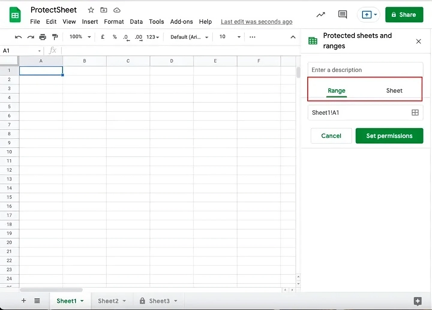
Step 3: You’ll see two options- Range and Sheet. Click Sheet.
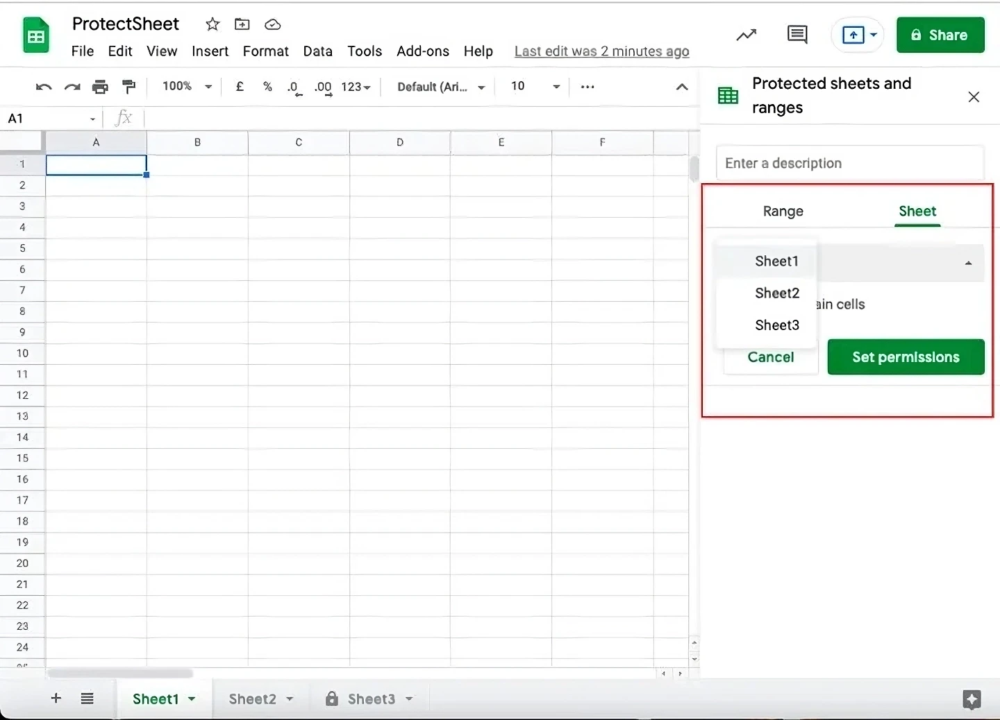
Step 4: If you have multiple sheets, then select the sheet you want to protect from the dropdown menu. You can also add a description to your protected sheet in the description box if needed.
Step 5: Now click Set permissions.
Step 6: In order to restrict editing permission, tick the option ‘Restrict who can edit the page’. In the dropdown menu, select the option according to your requirement.
If you want to restrict the editing permission to only you then select Only you.
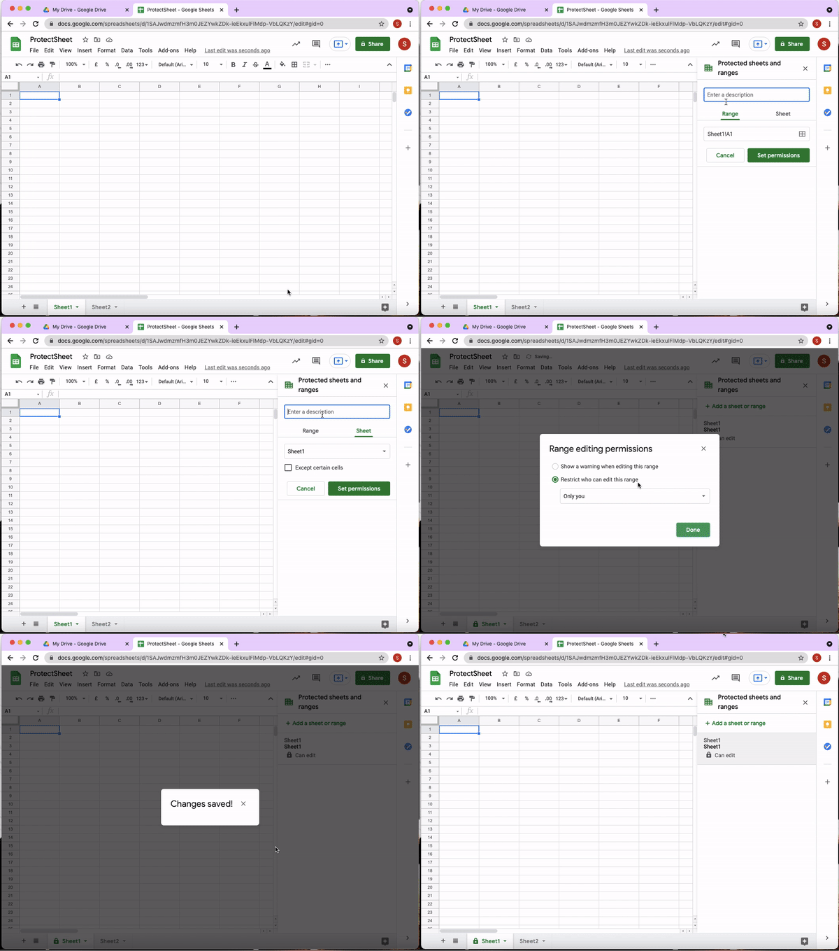
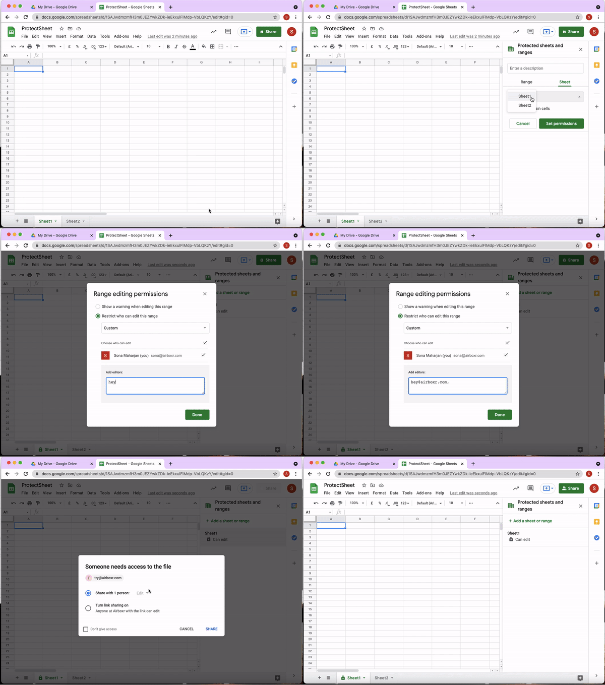
If you want to add more collaborators who can edit the data in your sheet, select Custom. Tick the email addresses you want to grant edit permission to if you’ve shared the sheet with them earlier. However, if the email address is not on the list then go to the Add editors field and type in the email address. If you want to add more than one email address, you can do so but make sure to separate them with a comma.
Step 7: Press Done. Now your entire sheet has been protected.
How to lock selected cells in Google Sheets
Sometimes you might want to prevent people from editing only specific cells in Google Sheets. In such cases, you could lock only selected cells.
Step 1: Go to Data -> Protected sheets and ranges. A box will open on the right.
Step 2: Click on Add a sheet or range.
Step 3: You’ll see two options- Range and Sheet. Click Range.
Step 4: You’ll see a default range pre-filled in a field. Change the range to the range of cells you want to protect. For instance, to protect cell A1 of Sheet 1, you can type Sheet1!A1.
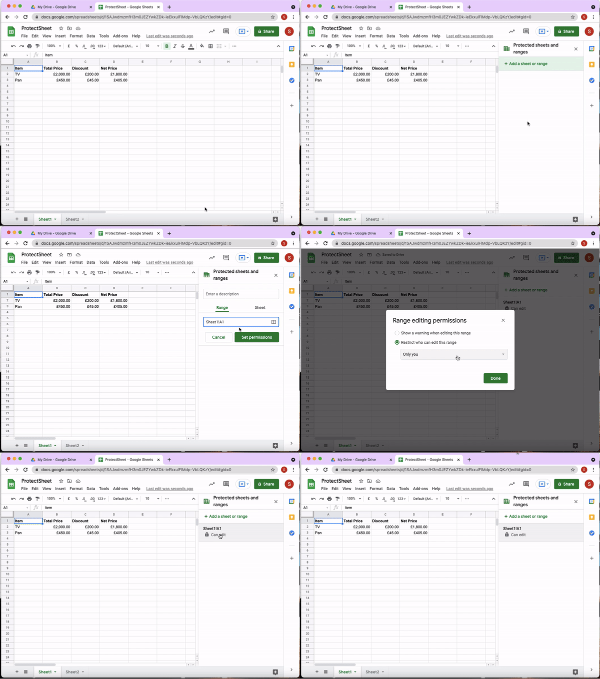
Similarly, you can protect a range of cells by adding a colon. Say you want to protect columns from C to D. You can type in Sheet1!C:D.
Then add a description to your protected range. This is optional but it is recommended to add a description as it can help you keep track of your protected range especially if you have multiple protected ranges.
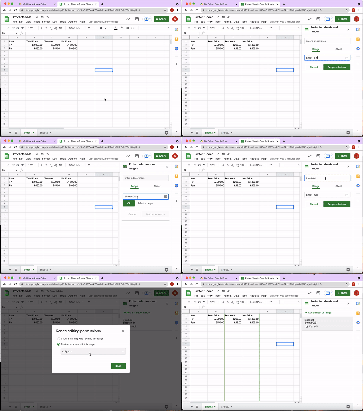
Step 5: Now click Set permissions.
Step 6: Then you can follow steps 6 and 7 from above.
Improve your DTC game. Sign up for weekly tips.
How to set soft warnings for editing cells
There might be a case where you might not want to totally restrict the editing of the cells. Instead, you might want to show a warning stating that specific cells are important and should not be changed before anyone tries editing them. In order to add such warnings, you can follow these steps.
Step 1: Go to Data → Protected sheets and ranges. A box will open on the right.
Step 2: Click on Add a sheet or range.
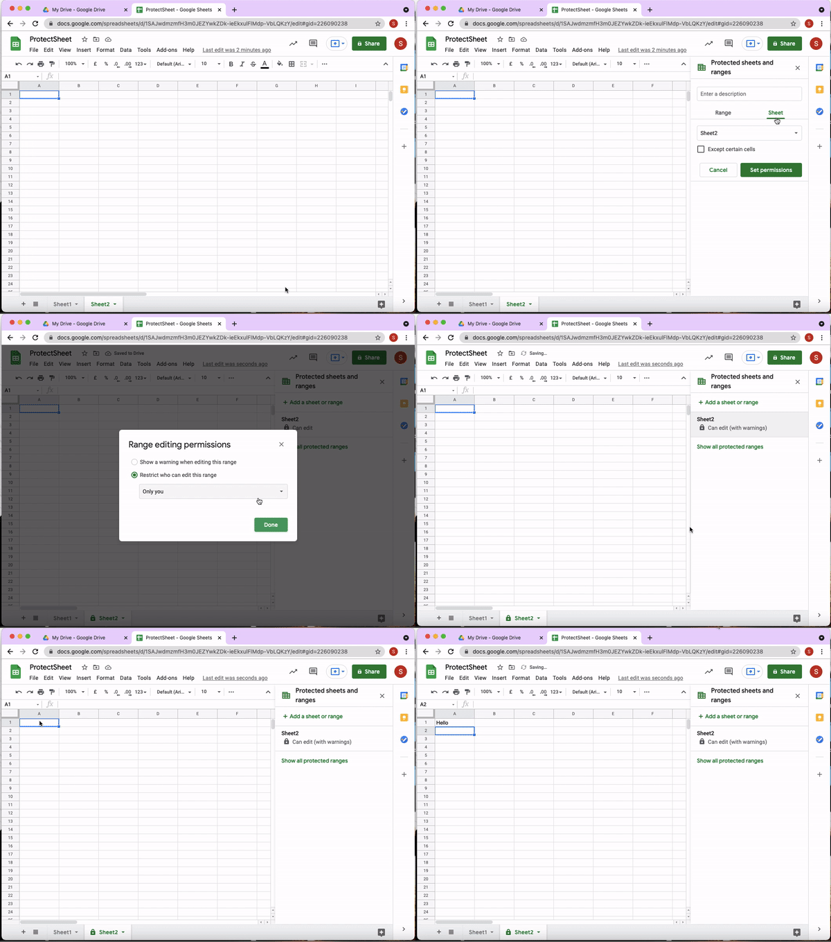
Step 3: You’ll see two options- Range and Sheet. Click either of the options depending on your preference. For this blog, we will be demonstrating setting a warning for the entire sheet. Therefore, select Sheet.
Step 4: If you have multiple sheets, then select the sheet you want to protect from the dropdown menu. You can also add a description to your protected sheet in the description box if needed.
Step 5: Now click Set permissions.
Step 6: Then tick the option ‘Show a warning when editing this page'.
Step 7: Press Done.
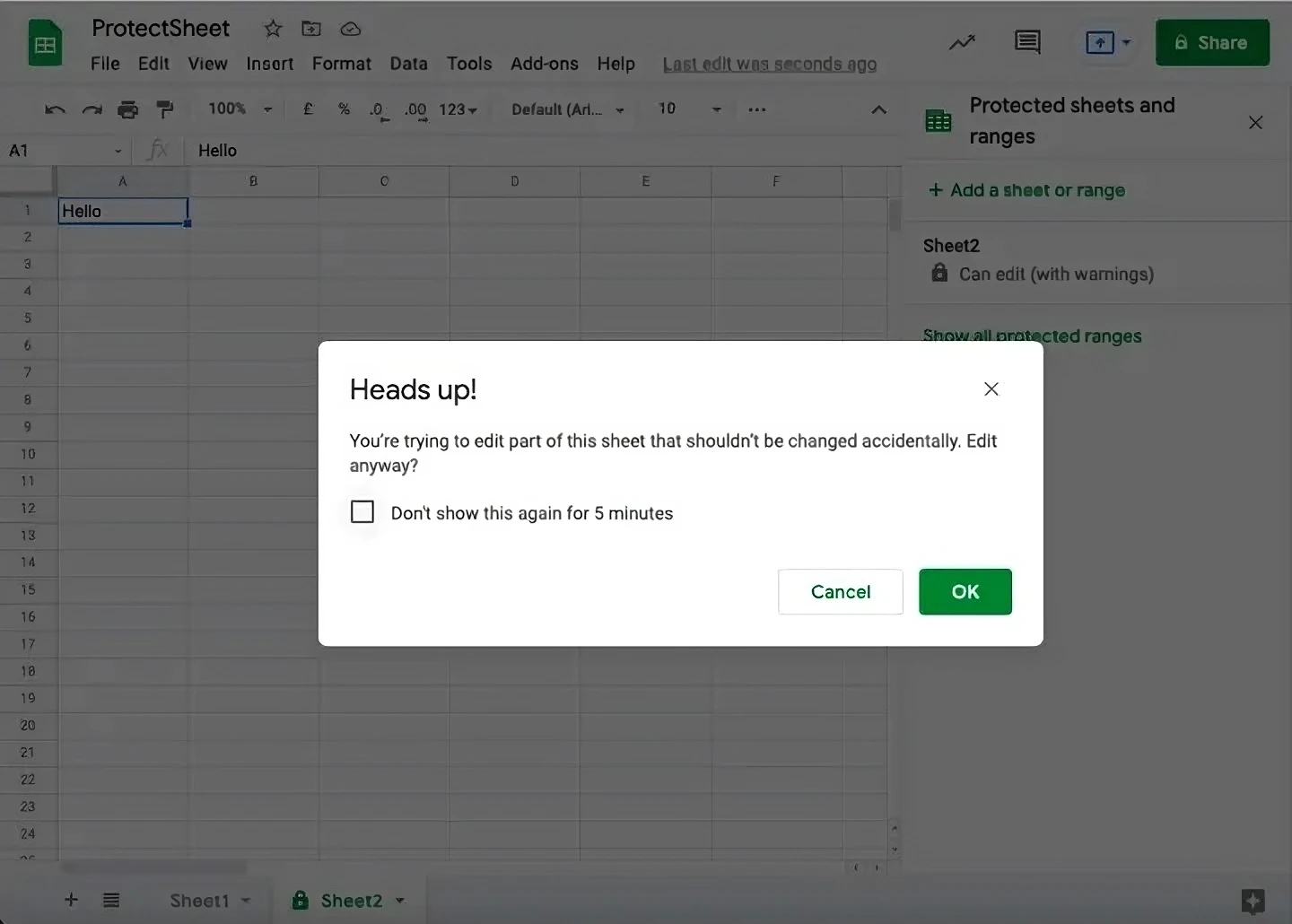
Now you can try editing the sheet to see a warning message.
How to add an exception to sheet protections
You can also exempt a few cells while protecting your sheet. That way even if the sheet is protected, people would still be able to make changes to specific cells as per the requirement.
Step 1: Go to Data → Protected sheets and ranges. A box will open on the right.
Step 2: Click on Add a sheet or range.
Step 3: You’ll see two options- Range and Sheet. Click Sheet.
Step 4: If you have multiple sheets, then select the sheet you want to protect from the dropdown menu. You can also add a description to your protected sheet in the description box if needed.
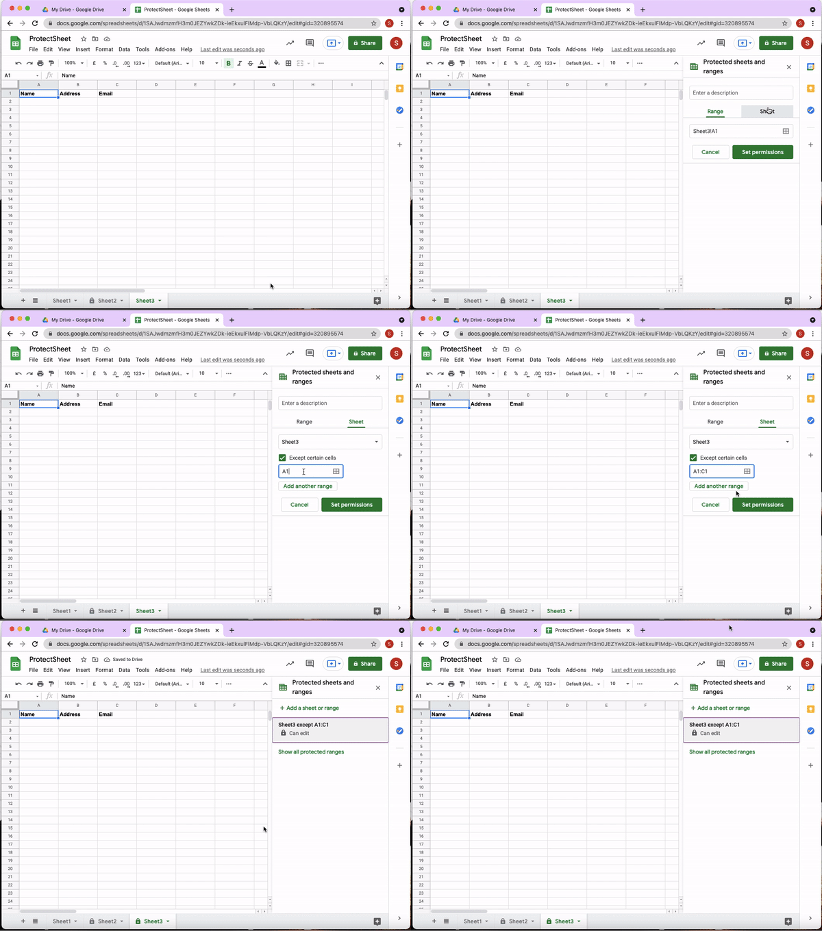
Step 5: Right below the sheet dropdown menu put a tick on Except certain cells.
Step 6: Now you can specify the cells or a range that you would like to exempt from protection. You can also press Add another range if you want to add multiple ranges.
Step 7: Once done, click Set permissions.
Step 8: Follow steps 6 and 7 from the section ‘How to protect your entire sheet in Google Sheets’.
How to remove protection from Google Sheets
Now you know how to protect sheets and ranges. But what if you want to remove the protection. In order to do so, you can go through these steps.
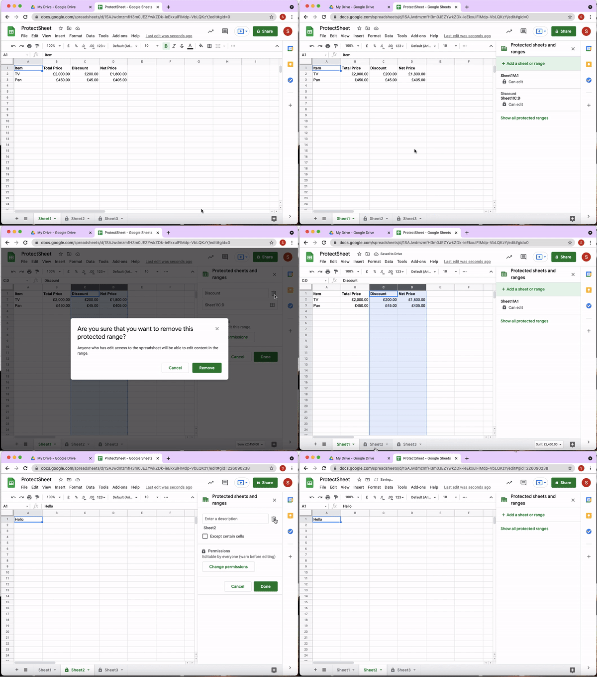
Step 1: Go to Data → Protected sheets and ranges.
Step 2: You’ll see all the protections you’ve added to the sheet on your right.
Step 3: Select the protection you want to delete.
Step 4: At the right of the description, you’ll see a delete icon. Click on that icon.
Step 5: Press Remove.
Now that you have learned how to protect your sheets and cells, you can add an extra layer of security to your important spreadsheets before sharing them with your peers and make them more secured. However, it is important to note that if a user makes a copy of your sheet, then they will be able to edit all the protected sheets and cells on the copied version. Having said that, your original sheet will still remain protected.


